Código
library(dplyr)
library(lubridate)
library(arrow)
library(zendown) # https://rfsaldanha.github.io/zendown/A pesquisa em clima e saúde tradicionalmente representa a exposição ambiental usando variáveis meteorológicas nominais, como temperatura média ou precipitação total, incluídas como covariáveis contínuas em modelos epidemiológicos. Embora esses indicadores sejam amplamente disponíveis e simples de implementar, muitas vezes representam de forma limitada condições persistentes, extremas e acima de limiares pelas quais a variabilidade e a mudança climática afetam a saúde humana. Muitos impactos em saúde são causados por eventos climáticos discretos, como ondas de calor, ondas de frio, chuva prolongada e períodos secos, cujos efeitos dependem de duração, intensidade e agrupamento temporal, não apenas de condições médias.
Proponho aqui um método para calcular, para cada município brasileiro, um conjunto mensal ou semanal de indicadores climáticos baseados em eventos e normais climatológicas.
Com pressa? Vá direto para a seção de baixar ;-)
Uma normal climatológica pode ser calculada com dados de diferentes fontes, incluindo sensores de sensoriamento remoto e “médias de área ou pontos em bases em grade” (WMO 2017). Algumas bases climatológicas em grade estão disponíveis para o território brasileiro, incluindo o ERA5-Land do Copernicus (Muñoz-Sabater et al. 2021) e a base BR-DWGD (Xavier et al. 2022), oferecendo vários indicadores climatológicos em séries longas e com atualizações contínuas.
Alguns métodos de pesquisa exigem que dados climáticos sejam agregados nas mesmas unidades espaciais e temporais de outros dados usados em modelos estatísticos, procedimento comum em estudos de epidemiologia e economia. Para lidar com essa necessidade, dados espaciais em grade podem ser agregados usando estatísticas zonais (Saldanha et al. 2024).
Para esta base, foram usadas estatísticas zonais climáticas do ERA5-Land para municípios brasileiros, descritas aqui, para calcular normais climatológicas e indicadores de eventos mensais e semanais.
Para calcular os indicadores baseados em eventos e as normais climatológicas, foi criado um pacote R chamado {climindi}. O pacote fornece funções auxiliares para calcular normais climatológicas e indicadores climáticos baseados em eventos de forma tidy.
O pacote {climindi} calcula média, percentil 10 e percentil 90 como normais climatológicas.
Foram calculadas duas normais climatológicas: 1961-1990 e 1981-2010.
Considerando cada normal climatológica, um conjunto de indicadores baseados em eventos foi calculado com o pacote {climindi} para temperatura máxima e mínima, precipitação total, umidade relativa média e velocidade média do vento.
Para cada indicador climático, foram calculados indicadores padrão e indicadores específicos.
count Contagem de pontos de dadosmean Valor médiomedian Medianasd Desvio padrãose Erro padrãomax Valor máximomin Valor mínimop10 Percentil 10p25 25th percentilep75 75th percentilep90 Percentil 90rs3 Períodos chuvosos: contagem de ocorrências com 3 e 5 ou mais dias consecutivos com chuva acima do valor médio da normal climatológicap_1 Contagem de dias com precipitação acima de 1mmp_5 Contagem de dias com precipitação acima de 5mmp_10 Contagem de dias com precipitação acima de 10mmp_50 Contagem de dias com precipitação acima de 50mmp_100 Contagem de dias com precipitação acima de 100mmd_3 Contagem de sequências de 3 dias ou mais sem precipitaçãod_5 Contagem de sequências de 5 dias ou mais sem precipitaçãod_10 Contagem de sequências de 10 dias ou mais sem precipitaçãod_15 Contagem de sequências de 15 dias ou mais sem precipitaçãod_20 Contagem de sequências de 20 dias ou mais sem precipitaçãod_25 Contagem de sequências de 25 dias ou mais sem precipitaçãohw3 Contagem de ocorrências de ondas de calor com 3 ou mais dias consecutivos com temperatura máxima acima da normal climatológica mais 5 graus Celsiushw5 Contagem de ocorrências de ondas de calor com 5 ou mais dias consecutivos com temperatura máxima acima da normal climatológica mais 5 graus Celsiushot_days Contagem de dias quentes, quando a temperatura máxima está acima do percentil 90 da normalt_25 Contagem de dias com temperaturas maiores ou iguais a 25 graus Celsiust_30 Contagem de dias com temperaturas maiores ou iguais a 30 graus Celsiust_35 Contagem de dias com temperaturas maiores ou iguais a 35 graus Celsiust_40 Contagem de dias com temperaturas maiores ou iguais a 40 graus Celsiuscw3 Contagem de ocorrências de ondas de frio com 3 ou mais dias consecutivos com temperatura mínima abaixo da normal climatológica menos 5 graus Celsiuscw5 Contagem de ocorrências de ondas de frio com 5 ou mais dias consecutivos com temperatura mínima abaixo da normal climatológica menos 5 graus Celsiuscold_days Contagem de dias frios, quando a temperatura mínima está abaixo do percentil 10 da normalt_0 Contagem de dias com temperaturas menores ou iguais a 0 graus Celsiust_5 Contagem de dias com temperaturas menores ou iguais a 5 graus Celsiust_10 Contagem de dias com temperaturas menores ou iguais a 10 graus Celsiust_15 Contagem de dias com temperaturas menores ou iguais a 15 graus Celsiust_20 Contagem de dias com temperaturas menores ou iguais a 20 graus Celsiusds3 Contagem de ocorrências de períodos secos com 3 ou mais dias consecutivos com umidade relativa abaixo da normal climatológica menos 10%ds5 Contagem de ocorrências de períodos secos com 5 ou mais dias consecutivos com umidade relativa abaixo da normal climatológica menos 10%ws3 Contagem de ocorrências de períodos úmidos com 3 ou mais dias consecutivos com umidade relativa acima da normal climatológica mais 10%ws5 Contagem de ocorrências de períodos úmidos com 5 ou mais dias consecutivos com umidade relativa acima da normal climatológica mais 10%dry_days Contagem de dias secos, quando a umidade relativa está abaixo do percentil 10 da normalwet_days Contagem de dias úmidos, quando a umidade relativa está acima do percentil 90 da normalh_21_30 Contagem de dias com umidade relativa entre 21% and 30% (nível de atenção)h_12_20 Contagem de dias com umidade relativa entre 12% and 20% (nível de alerta)h_11 Contagem de dias com umidade relativa abaixo de 12% (nível de emergência)l_eto_3 Contagem de sequências de 3 ou mais dias consecutivos com velocidade do vento abaixo da normal climatológica médial_eto_5 Contagem de sequências de 5 ou mais dias consecutivos com velocidade do vento abaixo da normal climatológica médiah_eto_3 Contagem de sequências de 3 ou mais dias consecutivos com velocidade do vento acima da normal climatológica médiah_eto_5 Contagem de sequências de 5 ou mais dias consecutivos com velocidade do vento acima da normal climatológica médiab1 Contagem de dias classificados como nível 1 na escala Beaufortb2 Contagem de dias classificados como nível 2 na escala Beaufortb3 Contagem de dias classificados como nível 3 na escala Beaufortb4 Contagem de dias classificados como nível 4 na escala Beaufortb5 Contagem de dias classificados como nível 5 na escala Beaufortb6 Contagem de dias classificados como nível 6 na escala Beaufortb7 Contagem de dias classificados como nível 7 na escala Beaufortb8 Contagem de dias classificados como nível 8 na escala Beaufortb9 Contagem de dias classificados como nível 9 na escala Beaufortb10 Contagem de dias classificados como nível 10 na escala Beaufortb11 Contagem de dias classificados como nível 11 na escala Beaufortb12 Contagem de dias classificados como nível 12 na escala BeaufortAs funções do pacote precisam dos dados em unidades específicas. Certifique-se de que seus dados estejam na unidade exigida antes de executar as funções.
O código usado para calcular esta base está disponível aqui.
As normais climatológicas e os indicadores baseados em eventos podem ser baixados do Zenodo nos formatos CSV e parquet. Clique no link abaixo para acessar e baixar os dados.
![]()
Também é possível baixar a base diretamente pelo R usando o pacote {zendown}.
Vamos verificar alguns resultados usando as bases mensais e a normal climatológica 1981-2010.
library(dplyr)
library(lubridate)
library(arrow)
library(zendown) # https://rfsaldanha.github.io/zendown/# Dados de 2024
tmax_data <- zen_file(15748125, "2m_temperature_max.parquet") |>
open_dataset() |>
filter(name == "2m_temperature_max_mean") |>
filter(code_muni == 3304557) |>
select(-name) |>
mutate(value = round(value - 273.15, digits = 2)) |>
collect()
# Normais climatológicas
tmax_normal <- zen_file(18612340, "tmax_monthly_normal_n1981_2010.parquet") |>
open_dataset() |>
filter(code_muni == 3304557) |>
collect()library(ggplot2)
library(tidyr)
# Preparar dados para o gráfico
tmax_normal_exp <- tmax_normal |>
mutate(date = as_date(paste0("2024-", month, "-01"))) |>
group_by(month) %>%
expand(
date = seq.Date(
floor_date(date, unit = "month"),
ceiling_date(date, unit = "month") - days(1),
by = "day"
),
normal_mean,
normal_p10,
normal_p90
) |>
pivot_longer(cols = starts_with("normal_")) |>
mutate(name = substr(name, 8, 100))
# Gráfico
ggplot() +
geom_line(data = tmax_data, aes(x = date, y = value)) +
geom_line(data = tmax_normal_exp, aes(x = date, y = value, color = name)) +
theme_bw() +
labs(
title = "Temperaturas máximas e normais climatológicas mensais",
subtitle = "Rio de Janeiro, RJ",
color = "Normal (1981-2010)",
x = "Data",
y = "graus Celsius"
) +
theme(legend.position = "bottom", legend.direction = "horizontal")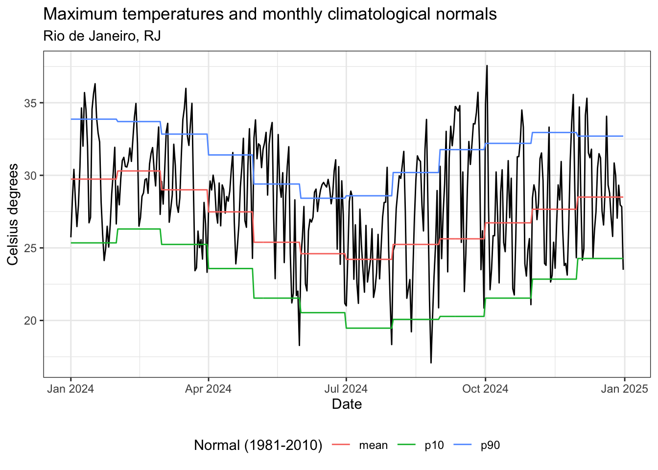
# Normais climatológicas
tmax_normal <- zen_file(18612340, "tmax_weekly_normal_n1981_2010.parquet") |>
  open_dataset() |>
  filter(code_muni == 3304557) |>
  collect()

tmax_normal_exp <- tmax_normal |>
  filter_out(week == 53) |>
  mutate(date = as.Date(paste(2024, week, 1, sep = "-"), "%Y-%U-%u")) |>
  group_by(week) %>%
  expand(
    date = seq.Date(
      floor_date(date, unit = "week"),
      ceiling_date(date, unit = "week") - days(1),
      by = "day"
    ),
    normal_mean,
    normal_p10,
    normal_p90
  ) |>
  pivot_longer(cols = starts_with("normal_")) |>
  mutate(name = substr(name, 8, 100))

# Gráfico
ggplot() +
  geom_line(data = tmax_data, aes(x = date, y = value)) +
  geom_line(data = tmax_normal_exp, aes(x = date, y = value, color = name)) +
  theme_bw() +
  labs(
    title = "Temperaturas máximas e normais climatológicas semanais, 2024",
    subtitle = "Rio de Janeiro, RJ",
    color = "Normal (1981-2010)",
    x = "Data",
    y = "graus Celsius"
  ) +
  theme(legend.position = "bottom", legend.direction = "horizontal")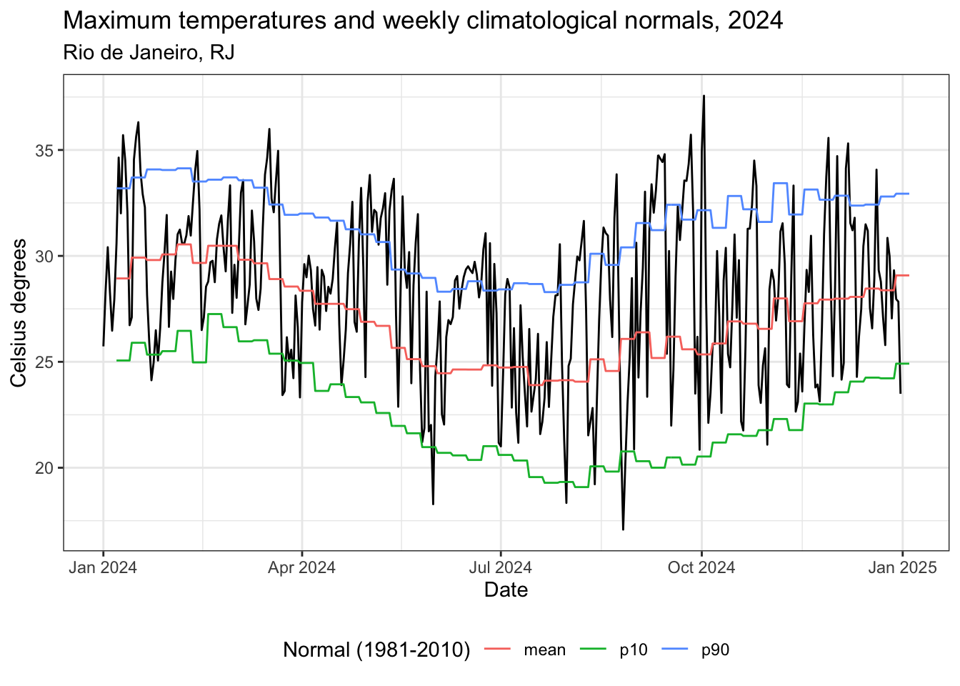
library(gt)

# Carregar indicadores baseados em eventos e filtrar o ano
zen_file(18612340, "tmax_monthly_indi_n1981_2010.parquet") |>
  open_dataset() |>
  filter(code_muni == 3304557) |>
  filter(year == 2024) |>
  select(-code_muni, -year) |>
  collect() |>
  gt() |>
  fmt_number(
    columns = where(is.double),
    decimals = 2,
    use_seps = FALSE
)| month | count | normal_mean | normal_p10 | normal_p90 | mean | median | sd | se | max | min | p10 | p25 | p75 | p90 | hw3 | hw5 | hot_days | t_25 | t_30 | t_35 | t_40 |
|---|---|---|---|---|---|---|---|---|---|---|---|---|---|---|---|---|---|---|---|---|---|
| 1.00 | 31 | 29.74 | 25.35 | 33.87 | 29.84 | 28.73 | 3.69 | 0.66 | 36.31 | 24.13 | 25.73 | 26.62 | 32.60 | 34.64 | 0 | 0 | 7 | 29 | 15 | 3 | 0 |
| 2.00 | 29 | 30.30 | 26.30 | 33.70 | 30.46 | 30.61 | 2.01 | 0.37 | 34.95 | 26.50 | 27.84 | 29.26 | 31.68 | 32.67 | 0 | 0 | 2 | 29 | 17 | 0 | 0 |
| 3.00 | 31 | 29.00 | 25.24 | 32.84 | 29.31 | 28.65 | 3.68 | 0.66 | 35.99 | 23.32 | 24.23 | 26.72 | 32.42 | 33.84 | 0 | 0 | 7 | 27 | 13 | 1 | 0 |
| 4.00 | 30 | 27.48 | 23.58 | 31.40 | 28.50 | 28.95 | 2.22 | 0.41 | 33.21 | 23.90 | 26.29 | 26.79 | 29.58 | 30.79 | 0 | 0 | 3 | 28 | 7 | 0 | 0 |
| 5.00 | 31 | 25.39 | 21.54 | 29.40 | 28.68 | 30.18 | 4.41 | 0.79 | 33.82 | 18.28 | 21.87 | 25.87 | 32.15 | 32.96 | 12 | 9 | 16 | 23 | 16 | 0 | 0 |
| 6.00 | 30 | 24.60 | 20.54 | 28.42 | 27.47 | 28.22 | 2.59 | 0.47 | 31.07 | 21.18 | 23.74 | 26.32 | 29.30 | 29.78 | 0 | 0 | 14 | 24 | 3 | 0 | 0 |
| 7.00 | 31 | 24.21 | 19.47 | 28.59 | 24.68 | 24.34 | 2.89 | 0.52 | 30.55 | 18.34 | 21.29 | 22.62 | 26.86 | 28.20 | 0 | 0 | 2 | 14 | 1 | 0 | 0 |
| 8.00 | 31 | 25.24 | 20.08 | 30.19 | 26.43 | 27.53 | 4.34 | 0.78 | 33.85 | 17.08 | 20.87 | 22.94 | 29.88 | 31.34 | 3 | 0 | 7 | 20 | 7 | 0 | 0 |
| 9.00 | 30 | 25.62 | 20.28 | 31.77 | 30.09 | 31.61 | 4.37 | 0.80 | 35.72 | 20.85 | 23.49 | 26.48 | 33.50 | 34.61 | 16 | 16 | 15 | 24 | 19 | 1 | 0 |
| 10.00 | 31 | 26.73 | 21.54 | 32.20 | 27.53 | 27.08 | 4.33 | 0.78 | 37.56 | 21.09 | 22.19 | 24.32 | 30.69 | 33.32 | 3 | 0 | 5 | 21 | 10 | 1 | 0 |
| 11.00 | 30 | 27.66 | 22.85 | 32.95 | 27.72 | 28.18 | 3.52 | 0.64 | 35.57 | 22.65 | 23.55 | 24.03 | 29.57 | 31.72 | 0 | 0 | 3 | 21 | 7 | 1 | 0 |
| 12.00 | 31 | 28.50 | 24.27 | 32.70 | 29.04 | 28.78 | 3.13 | 0.56 | 35.31 | 23.49 | 24.94 | 27.07 | 31.20 | 34.07 | 0 | 0 | 4 | 27 | 11 | 1 | 0 |
# Dados de 2025
tmin_data <- zen_file(18257037, "2m_temperature_min.parquet") |>
  open_dataset() |>
  filter(name == "2m_temperature_min_mean") |>
  filter(code_muni == 4218954) |>
  select(-name) |>
  mutate(value = round(value - 273.15, digits = 2)) |>
  collect()

# Normais climatológicas
tmin_normal <- zen_file(18612340, "tmin_monthly_normal_n1981_2010.parquet") |>
  open_dataset() |>
  filter(code_muni == 4218954) |>
collect()library(ggplot2)
library(tidyr)
# Preparar dados para o gráfico
tmin_normal_exp <- tmin_normal |>
mutate(date = as_date(paste0("2025-", month, "-01"))) |>
group_by(month) %>%
expand(
date = seq.Date(
floor_date(date, unit = "month"),
ceiling_date(date, unit = "month") - days(1),
by = "day"
),
normal_mean,
normal_p10,
normal_p90
) |>
pivot_longer(cols = starts_with("normal_")) |>
mutate(name = substr(name, 8, 100))
# Gráfico
ggplot() +
geom_line(data = tmin_data, aes(x = date, y = value)) +
geom_line(data = tmin_normal_exp, aes(x = date, y = value, color = name)) +
theme_bw() +
labs(
title = "Temperaturas mínimas e normais climatológicas mensais, 2025",
subtitle = "Urupema, SC",
color = "Normal (1981-2010)",
x = "Data",
y = "graus Celsius"
) +
theme(legend.position = "bottom", legend.direction = "horizontal")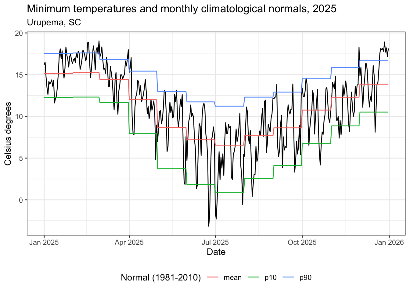
library(gt)

# Carregar indicadores baseados em eventos e filtrar o ano
zen_file(18612340, "tmin_monthly_indi_n1981_2010.parquet") |>
  open_dataset() |>
  filter(code_muni == 4218954) |>
  filter(year == 2025) |>
  select(-code_muni, -year) |>
  collect() |>
  gt() |>
  fmt_number(
    columns = where(is.double),
    decimals = 2,
    use_seps = FALSE
)| month | count | normal_mean | normal_p10 | normal_p90 | mean | median | sd | se | max | min | p10 | p25 | p75 | p90 | cw3 | cw5 | cold_days | t_0 | t_5 | t_10 | t_15 | t_20 |
|---|---|---|---|---|---|---|---|---|---|---|---|---|---|---|---|---|---|---|---|---|---|---|
| 1.00 | 31 | 15.14 | 12.28 | 17.54 | 15.33 | 15.66 | 1.88 | 0.34 | 18.32 | 11.61 | 12.63 | 13.97 | 16.89 | 17.43 | 0 | 0 | 2 | 0 | 0 | 0 | 14 | 31 |
| 2.00 | 28 | 15.28 | 12.32 | 17.60 | 17.20 | 17.24 | 1.06 | 0.20 | 19.05 | 14.64 | 15.67 | 16.69 | 17.83 | 18.56 | 0 | 0 | 0 | 0 | 0 | 0 | 1 | 28 |
| 3.00 | 31 | 14.41 | 11.66 | 16.83 | 15.02 | 15.16 | 1.96 | 0.35 | 18.33 | 10.25 | 12.52 | 14.06 | 16.34 | 17.16 | 0 | 0 | 2 | 0 | 0 | 0 | 14 | 31 |
| 4.00 | 30 | 12.00 | 7.94 | 15.42 | 11.80 | 11.94 | 2.54 | 0.46 | 17.04 | 4.81 | 8.87 | 10.38 | 13.31 | 14.50 | 0 | 0 | 2 | 0 | 1 | 5 | 27 | 30 |
| 5.00 | 31 | 8.68 | 3.73 | 13.00 | 9.65 | 10.30 | 2.85 | 0.51 | 13.15 | 1.84 | 6.40 | 8.66 | 11.44 | 12.66 | 0 | 0 | 2 | 0 | 2 | 13 | 31 | 31 |
| 6.00 | 30 | 7.21 | 1.81 | 11.74 | 7.06 | 7.74 | 3.74 | 0.68 | 11.59 | −3.16 | 1.67 | 5.50 | 9.87 | 10.89 | 0 | 0 | 4 | 2 | 7 | 25 | 30 | 30 |
| 7.00 | 31 | 6.56 | 0.90 | 11.22 | 5.17 | 5.52 | 3.35 | 0.60 | 10.39 | −2.30 | 0.03 | 2.83 | 7.95 | 8.77 | 3 | 0 | 4 | 3 | 12 | 30 | 31 | 31 |
| 8.00 | 31 | 7.69 | 2.54 | 12.31 | 7.52 | 7.81 | 3.04 | 0.55 | 12.17 | 0.38 | 3.04 | 5.44 | 9.82 | 11.12 | 0 | 0 | 2 | 0 | 7 | 24 | 31 | 31 |
| 9.00 | 30 | 8.63 | 4.13 | 12.91 | 8.60 | 8.45 | 3.13 | 0.57 | 13.89 | 3.32 | 5.15 | 6.06 | 10.88 | 12.47 | 0 | 0 | 2 | 0 | 3 | 18 | 30 | 30 |
| 10.00 | 31 | 10.75 | 6.74 | 14.51 | 10.38 | 10.20 | 2.65 | 0.48 | 14.60 | 4.17 | 6.60 | 8.74 | 12.73 | 13.30 | 0 | 0 | 4 | 0 | 1 | 14 | 31 | 31 |
| 11.00 | 30 | 12.30 | 8.86 | 15.87 | 11.80 | 12.20 | 2.47 | 0.45 | 18.30 | 7.40 | 9.00 | 9.66 | 13.66 | 14.09 | 0 | 0 | 3 | 0 | 0 | 10 | 29 | 30 |
| 12.00 | 31 | 13.86 | 10.52 | 16.73 | 15.01 | 15.00 | 2.74 | 0.49 | 18.92 | 8.10 | 11.12 | 13.36 | 17.62 | 18.15 | 0 | 0 | 1 | 0 | 0 | 1 | 16 | 31 |
# Dados de 2025
rh_data <- zen_file(18392587, "rh_mean_mean_2025.parquet") |>
  open_dataset() |>
  filter(name == "rh_mean_mean") |>
  filter(code_muni == 5001102) |>
  select(-name) |>
  collect()

# Normais climatológicas
rh_normal <- zen_file(18612340, "rh_normal_monthly_n1981_2010.parquet") |>
  open_dataset() |>
  filter(code_muni == 5001102) |>
collect()library(ggplot2)
library(tidyr)
# Preparar dados para o gráfico
rh_normal_exp <- rh_normal |>
mutate(date = as_date(paste0("2025-", month, "-01"))) |>
group_by(month) %>%
expand(
date = seq.Date(
floor_date(date, unit = "month"),
ceiling_date(date, unit = "month") - days(1),
by = "day"
),
normal_mean,
normal_p10,
normal_p90
) |>
pivot_longer(cols = starts_with("normal_")) |>
mutate(name = substr(name, 8, 100))
# Gráfico
ggplot() +
geom_line(data = rh_data, aes(x = date, y = value)) +
geom_line(data = rh_normal_exp, aes(x = date, y = value, color = name)) +
theme_bw() +
labs(
title = "Umidade relativa e normais climatológicas mensais, 2025",
subtitle = "Aquidauana, MS",
color = "Normal (1981-2010)",
x = "Data",
y = "%"
) +
theme(legend.position = "bottom", legend.direction = "horizontal")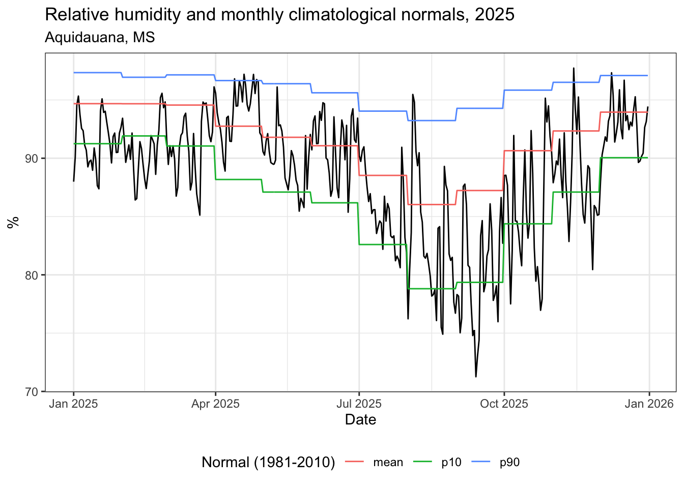
library(gt)

# Carregar indicadores baseados em eventos e filtrar o ano
zen_file(18612340, "rh_indi_monthly_n1981_2010.parquet") |>
  open_dataset() |>
  filter(code_muni == 5001102) |>
  filter(year == 2025) |>
  select(-code_muni, -year) |>
  collect() |>
  gt() |>
  fmt_number(
    columns = where(is.double),
    decimals = 2,
    use_seps = FALSE
)| month | count | normal_mean | normal_p10 | normal_p90 | mean | median | sd | se | max | min | p10 | p25 | p75 | p90 | ds3 | ds5 | ws3 | ws5 | dry_days | wet_days | h_21_30 | h_12_20 | h_11 |
|---|---|---|---|---|---|---|---|---|---|---|---|---|---|---|---|---|---|---|---|---|---|---|---|
| 1.00 | 31 | 94.68 | 91.25 | 97.34 | 91.45 | 91.21 | 2.17 | 0.39 | 95.33 | 87.38 | 88.97 | 89.84 | 92.85 | 94.07 | 0 | 0 | 31 | 31 | 16 | 0 | 0 | 0 | 0 |
| 2.00 | 28 | 94.67 | 91.91 | 96.94 | 90.79 | 90.98 | 2.45 | 0.46 | 95.57 | 86.42 | 87.98 | 89.07 | 92.00 | 94.48 | 0 | 0 | 28 | 28 | 20 | 0 | 0 | 0 | 0 |
| 3.00 | 31 | 94.56 | 91.05 | 97.15 | 90.96 | 91.42 | 2.82 | 0.51 | 96.12 | 85.12 | 86.95 | 89.34 | 92.72 | 94.63 | 0 | 0 | 31 | 31 | 13 | 0 | 0 | 0 | 0 |
| 4.00 | 30 | 92.75 | 88.18 | 96.66 | 94.16 | 94.48 | 2.23 | 0.41 | 97.20 | 88.90 | 91.43 | 92.64 | 96.09 | 96.76 | 0 | 0 | 30 | 30 | 0 | 4 | 0 | 0 | 0 |
| 5.00 | 31 | 91.80 | 87.10 | 96.39 | 89.74 | 89.85 | 2.40 | 0.43 | 96.11 | 85.46 | 86.56 | 87.96 | 91.22 | 92.33 | 0 | 0 | 31 | 31 | 4 | 0 | 0 | 0 | 0 |
| 6.00 | 30 | 91.07 | 86.18 | 95.61 | 91.15 | 91.31 | 2.67 | 0.49 | 94.76 | 85.37 | 87.23 | 89.86 | 93.40 | 94.03 | 0 | 0 | 30 | 30 | 1 | 0 | 0 | 0 | 0 |
| 7.00 | 31 | 88.53 | 82.60 | 94.04 | 85.44 | 85.26 | 3.06 | 0.55 | 90.98 | 80.61 | 81.60 | 83.28 | 87.24 | 90.24 | 0 | 0 | 31 | 31 | 6 | 0 | 0 | 0 | 0 |
| 8.00 | 31 | 86.03 | 78.81 | 93.23 | 82.89 | 81.60 | 5.53 | 0.99 | 95.47 | 74.91 | 76.23 | 78.52 | 86.29 | 90.47 | 0 | 0 | 31 | 31 | 9 | 2 | 0 | 0 | 0 |
| 9.00 | 30 | 87.23 | 79.36 | 94.28 | 80.01 | 79.12 | 4.54 | 0.83 | 87.78 | 71.26 | 74.75 | 76.57 | 83.64 | 86.14 | 5 | 5 | 30 | 30 | 16 | 0 | 0 | 0 | 0 |
| 10.00 | 31 | 90.65 | 84.38 | 95.84 | 85.64 | 84.62 | 5.23 | 0.94 | 95.15 | 76.96 | 79.13 | 82.03 | 89.62 | 92.37 | 3 | 0 | 31 | 31 | 13 | 0 | 0 | 0 | 0 |
| 11.00 | 30 | 92.34 | 87.10 | 96.51 | 88.29 | 87.95 | 3.74 | 0.68 | 97.73 | 80.45 | 84.79 | 85.75 | 90.22 | 92.39 | 0 | 0 | 30 | 30 | 12 | 1 | 0 | 0 | 0 |
| 12.00 | 31 | 93.95 | 90.05 | 97.09 | 92.69 | 92.77 | 2.12 | 0.38 | 97.33 | 88.03 | 90.16 | 91.42 | 93.66 | 95.40 | 0 | 0 | 31 | 31 | 3 | 1 | 0 | 0 | 0 |
# Dados de 2025
prec_data <- zen_file(18257037, "total_precipitation_sum.parquet") |>
  open_dataset() |>
  filter(name == "total_precipitation_sum_mean") |>
  filter(code_muni == 1600204) |>
  mutate(value = round(value * 1000, digits = 2)) |>
  select(-name) |>
  collect()

# Normais climatológicas
prec_normal <- zen_file(18612340, "prec_monthly_normal_n1981_2010.parquet") |>
  open_dataset() |>
  filter(code_muni == 1600204) |>
collect()library(ggplot2)
library(tidyr)
# Preparar dados para o gráfico
prec_normal_exp <- prec_normal |>
mutate(date = as_date(paste0("2025-", month, "-01"))) |>
group_by(month) %>%
expand(
date = seq.Date(
floor_date(date, unit = "month"),
ceiling_date(date, unit = "month") - days(1),
by = "day"
),
normal_mean,
normal_p10,
normal_p90
) |>
pivot_longer(cols = starts_with("normal_")) |>
mutate(name = substr(name, 8, 100))
# Gráfico
ggplot() +
geom_line(data = prec_data, aes(x = date, y = value)) +
geom_line(data = prec_normal_exp, aes(x = date, y = value, color = name)) +
theme_bw() +
labs(
title = "Precipitação e normais climatológicas mensais, 2025",
subtitle = "Calçoene, AP",
color = "Normal (1981-2010)",
x = "Data",
y = "mm"
) +
theme(legend.position = "bottom", legend.direction = "horizontal")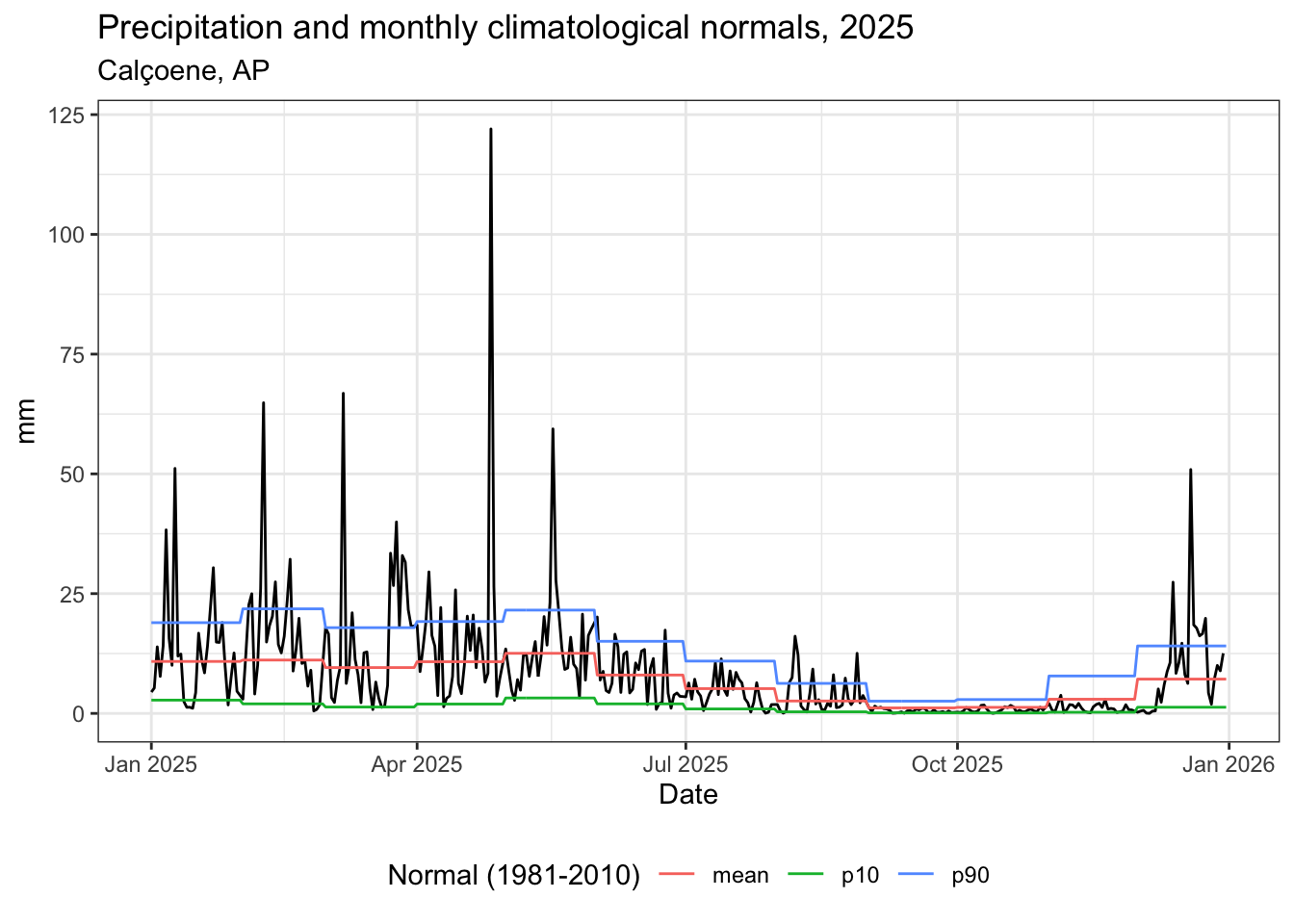
library(gt)

# Carregar indicadores baseados em eventos e filtrar o ano
zen_file(18612340, "prec_monthly_indi_n1981_2010.parquet") |>
  open_dataset() |>
  filter(code_muni == 5001102) |>
  filter(year == 2025) |>
  select(-code_muni, -year) |>
  collect() |>
  gt() |>
  fmt_number(
    columns = where(is.double),
    decimals = 2,
    use_seps = FALSE
)| month | count | normal_mean | normal_p10 | normal_p90 | mean | median | sd | se | max | min | p10 | p25 | p75 | p90 | rs3 | rs5 | p_1 | p_5 | p_10 | p_50 | p_100 | d_3 | d_5 | d_10 | d_15 | d_20 | d_25 |
|---|---|---|---|---|---|---|---|---|---|---|---|---|---|---|---|---|---|---|---|---|---|---|---|---|---|---|---|
| 1.00 | 30 | 8.68 | 0.47 | 19.71 | 3.15 | 1.77 | 3.63 | 0.66 | 14.70 | 0.13 | 0.34 | 0.79 | 4.00 | 7.55 | 0 | 0 | 21 | 7 | 2 | 0 | 0 | 0 | 0 | 0 | 0 | 0 | 0 |
| 2.00 | 27 | 6.64 | 0.43 | 15.06 | 3.17 | 2.28 | 3.97 | 0.76 | 19.15 | 0.07 | 0.29 | 0.75 | 3.85 | 6.93 | 3 | 0 | 19 | 5 | 1 | 0 | 0 | 0 | 0 | 0 | 0 | 0 | 0 |
| 3.00 | 30 | 5.71 | 0.25 | 13.44 | 2.10 | 1.17 | 2.58 | 0.47 | 11.25 | 0.02 | 0.07 | 0.37 | 3.06 | 4.48 | 0 | 0 | 17 | 2 | 1 | 0 | 0 | 0 | 0 | 0 | 0 | 0 | 0 |
| 4.00 | 29 | 3.19 | 0.00 | 10.02 | 5.30 | 2.90 | 5.95 | 1.10 | 18.28 | 0.06 | 0.22 | 0.60 | 8.44 | 15.37 | 5 | 5 | 19 | 11 | 7 | 0 | 0 | 0 | 0 | 0 | 0 | 0 | 0 |
| 5.00 | 30 | 2.85 | 0.00 | 9.89 | 1.55 | 0.00 | 5.93 | 1.08 | 29.97 | 0.00 | 0.00 | 0.00 | 0.15 | 0.53 | 0 | 0 | 2 | 2 | 2 | 0 | 0 | 3 | 1 | 0 | 0 | 0 | 0 |
| 6.00 | 29 | 1.53 | 0.00 | 3.84 | 1.04 | 0.04 | 3.12 | 0.58 | 13.98 | 0.00 | 0.00 | 0.00 | 0.56 | 0.96 | 0 | 0 | 3 | 2 | 2 | 0 | 0 | 2 | 0 | 0 | 0 | 0 | 0 |
| 7.00 | 30 | 1.02 | 0.00 | 1.98 | 0.10 | 0.00 | 0.51 | 0.09 | 2.80 | 0.00 | 0.00 | 0.00 | 0.00 | 0.00 | 0 | 0 | 1 | 0 | 0 | 0 | 0 | 1 | 1 | 1 | 1 | 1 | 1 |
| 8.00 | 30 | 1.19 | 0.00 | 2.20 | 0.92 | 0.00 | 4.56 | 0.83 | 25.04 | 0.00 | 0.00 | 0.00 | 0.01 | 0.47 | 0 | 0 | 2 | 1 | 1 | 0 | 0 | 2 | 1 | 1 | 0 | 0 | 0 |
| 9.00 | 29 | 2.81 | 0.00 | 9.09 | 0.27 | 0.00 | 0.75 | 0.14 | 3.29 | 0.00 | 0.00 | 0.00 | 0.03 | 0.76 | 0 | 0 | 3 | 0 | 0 | 0 | 0 | 4 | 1 | 0 | 0 | 0 | 0 |
| 10.00 | 30 | 4.73 | 0.00 | 14.63 | 2.15 | 0.31 | 3.98 | 0.73 | 18.32 | 0.00 | 0.01 | 0.03 | 2.08 | 7.41 | 0 | 0 | 10 | 5 | 1 | 0 | 0 | 0 | 0 | 0 | 0 | 0 | 0 |
| 11.00 | 29 | 6.01 | 0.02 | 16.21 | 4.04 | 0.14 | 9.36 | 1.74 | 39.31 | 0.00 | 0.00 | 0.01 | 2.06 | 14.92 | 0 | 0 | 10 | 4 | 4 | 0 | 0 | 1 | 0 | 0 | 0 | 0 | 0 |
| 12.00 | 30 | 7.76 | 0.23 | 17.82 | 7.08 | 2.46 | 11.00 | 2.01 | 41.39 | 0.16 | 0.41 | 0.93 | 5.87 | 29.58 | 4 | 0 | 22 | 11 | 5 | 0 | 0 | 0 | 0 | 0 | 0 | 0 | 0 |
# Dados de 2025
ws_data <- zen_file(18390794, "wind_speed_mean_mean_2025.parquet") |>
  open_dataset() |>
  filter(name == "wind_speed_mean_mean") |>
  filter(code_muni == 1600204) |>
  select(-name) |>
  collect()

# Normais climatológicas
ws_normal <- zen_file(18612340, "ws_monthly_normal_n1981_2010.parquet") |>
  open_dataset() |>
  filter(code_muni == 1600204) |>
collect()library(ggplot2)
library(tidyr)
# Preparar dados para o gráfico
ws_normal_exp <- ws_normal |>
mutate(date = as_date(paste0("2025-", month, "-01"))) |>
group_by(month) %>%
expand(
date = seq.Date(
floor_date(date, unit = "month"),
ceiling_date(date, unit = "month") - days(1),
by = "day"
),
normal_mean,
normal_p10,
normal_p90
) |>
pivot_longer(cols = starts_with("normal_")) |>
mutate(name = substr(name, 8, 100))
# Gráfico
ggplot() +
geom_line(data = ws_data, aes(x = date, y = value)) +
geom_line(data = ws_normal_exp, aes(x = date, y = value, color = name)) +
theme_bw() +
labs(
title = "Velocidade do vento e normais climatológicas mensais, 2025",
subtitle = "Caetité, BA",
color = "Normal (1981-2010)",
x = "Data",
y = "m/s"
) +
theme(legend.position = "bottom", legend.direction = "horizontal")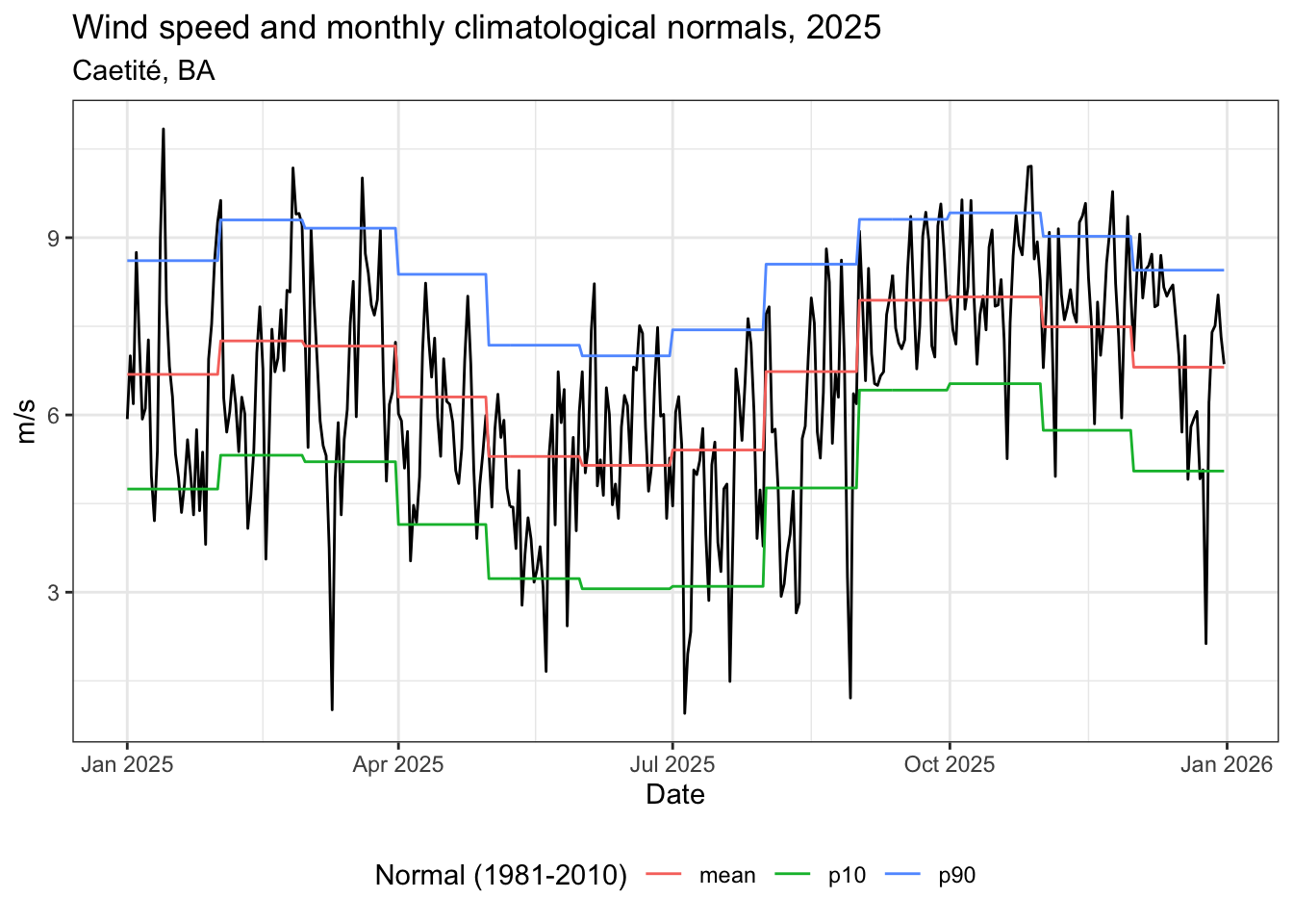
library(gt)

# Carregar indicadores baseados em eventos e filtrar o ano
zen_file(18612340, "ws_monthly_indi_n1981_2010.parquet") |>
  open_dataset() |>
  filter(code_muni == 5001102) |>
  filter(year == 2025) |>
  select(-code_muni, -year) |>
  collect() |>
  gt() |>
  fmt_number(
    columns = where(is.double),
    decimals = 2,
    use_seps = FALSE
)| month | count | normal_mean | normal_p10 | normal_p90 | mean | median | sd | se | max | min | p10 | p25 | p75 | p90 | l_u2_3 | l_u2_5 | h_u2_3 | h_u2_5 | b0 | b1 | b2 | b3 | b4 | b5 | b6 | b7 | b8 | b9 | b10 | b11 | b12 |
|---|---|---|---|---|---|---|---|---|---|---|---|---|---|---|---|---|---|---|---|---|---|---|---|---|---|---|---|---|---|---|---|
| 1.00 | 31 | 5.15 | 2.29 | 8.50 | 4.59 | 4.11 | 2.08 | 0.37 | 9.96 | 1.26 | 2.36 | 2.87 | 6.12 | 6.65 | 16 | 5 | 8 | 5 | 0.00 | 1.00 | 10.00 | 7.00 | 11.00 | 2.00 | 0.00 | 0.00 | 0.00 | 0.00 | 0.00 | 0.00 | 0.00 |
| 2.00 | 28 | 4.64 | 1.91 | 7.87 | 5.65 | 5.76 | 2.34 | 0.44 | 10.43 | 1.35 | 1.69 | 4.49 | 7.14 | 8.42 | 7 | 7 | 20 | 20 | 0.00 | 3.00 | 1.00 | 5.00 | 12.00 | 5.00 | 0.00 | 0.00 | 0.00 | 0.00 | 0.00 | 0.00 | 0.00 |
| 3.00 | 31 | 4.11 | 1.67 | 6.86 | 4.10 | 4.33 | 1.50 | 0.27 | 6.23 | 0.95 | 1.81 | 3.41 | 5.12 | 6.09 | 3 | 0 | 13 | 13 | 0.00 | 2.00 | 5.00 | 16.00 | 6.00 | 0.00 | 0.00 | 0.00 | 0.00 | 0.00 | 0.00 | 0.00 | 0.00 |
| 4.00 | 30 | 5.14 | 2.29 | 8.07 | 4.24 | 4.20 | 2.12 | 0.39 | 10.54 | 0.82 | 1.85 | 2.76 | 5.12 | 6.84 | 22 | 21 | 5 | 5 | 0.00 | 3.00 | 7.00 | 13.00 | 5.00 | 1.00 | 0.00 | 0.00 | 0.00 | 0.00 | 0.00 | 0.00 | 0.00 |
| 5.00 | 31 | 6.02 | 2.86 | 9.12 | 6.67 | 6.35 | 1.93 | 0.35 | 11.60 | 4.28 | 4.57 | 5.02 | 7.98 | 9.07 | 10 | 6 | 15 | 12 | 0.00 | 0.00 | 0.00 | 11.00 | 11.00 | 7.00 | 1.00 | 0.00 | 0.00 | 0.00 | 0.00 | 0.00 | 0.00 |
| 6.00 | 30 | 6.53 | 3.30 | 9.75 | 6.13 | 6.37 | 2.94 | 0.54 | 12.50 | 1.29 | 2.64 | 3.48 | 8.31 | 9.40 | 10 | 0 | 7 | 0 | 0.00 | 2.00 | 5.00 | 3.00 | 11.00 | 7.00 | 1.00 | 0.00 | 0.00 | 0.00 | 0.00 | 0.00 | 0.00 |
| 7.00 | 31 | 7.32 | 3.62 | 10.92 | 6.84 | 6.49 | 1.88 | 0.34 | 11.19 | 4.22 | 4.91 | 5.38 | 8.18 | 9.30 | 18 | 18 | 8 | 0 | 0.00 | 0.00 | 0.00 | 8.00 | 12.00 | 7.00 | 2.00 | 0.00 | 0.00 | 0.00 | 0.00 | 0.00 | 0.00 |
| 8.00 | 31 | 6.86 | 3.03 | 10.67 | 7.84 | 7.18 | 2.96 | 0.53 | 13.25 | 2.86 | 3.59 | 6.06 | 10.09 | 11.41 | 7 | 0 | 14 | 7 | 0.00 | 0.00 | 2.00 | 3.00 | 11.00 | 7.00 | 6.00 | 0.00 | 0.00 | 0.00 | 0.00 | 0.00 | 0.00 |
| 9.00 | 30 | 6.96 | 3.23 | 10.65 | 7.06 | 6.89 | 3.36 | 0.61 | 17.21 | 2.30 | 3.39 | 4.58 | 9.03 | 10.46 | 10 | 10 | 11 | 11 | 0.00 | 0.00 | 3.00 | 9.00 | 7.00 | 8.00 | 2.00 | 0.00 | 1.00 | 0.00 | 0.00 | 0.00 | 0.00 |
| 10.00 | 31 | 5.77 | 2.19 | 9.64 | 7.90 | 8.30 | 3.30 | 0.59 | 13.65 | 1.29 | 3.01 | 6.04 | 10.07 | 11.99 | 3 | 0 | 22 | 16 | 0.00 | 1.00 | 4.00 | 1.00 | 7.00 | 10.00 | 6.00 | 0.00 | 0.00 | 0.00 | 0.00 | 0.00 | 0.00 |
| 11.00 | 30 | 5.38 | 1.95 | 9.27 | 5.15 | 5.34 | 2.19 | 0.40 | 11.79 | 1.20 | 2.66 | 3.38 | 6.38 | 7.27 | 9 | 5 | 6 | 6 | 0.00 | 1.00 | 7.00 | 8.00 | 11.00 | 1.00 | 1.00 | 0.00 | 0.00 | 0.00 | 0.00 | 0.00 | 0.00 |
| 12.00 | 31 | 5.32 | 2.10 | 8.82 | 6.17 | 6.48 | 2.77 | 0.50 | 11.82 | 0.98 | 2.86 | 3.91 | 7.75 | 9.74 | 13 | 5 | 17 | 17 | 0.00 | 1.00 | 3.00 | 7.00 | 11.00 | 5.00 | 2.00 | 0.00 | 0.00 | 0.00 | 0.00 | 0.00 | 0.00 |
sessioninfo::session_info()─ Session info ───────────────────────────────────────────────────────────────
setting value
version R version 4.3.3 (2024-02-29)
os Ubuntu 24.04.4 LTS
system x86_64, linux-gnu
ui X11
language (EN)
collate C.UTF-8
ctype C.UTF-8
tz America/Sao_Paulo
date 2026-05-21
pandoc 3.1.3 @ /usr/bin/ (via rmarkdown)
quarto 1.8.26 @ /usr/local/bin/quarto
─ Packages ───────────────────────────────────────────────────────────────────
package * version date (UTC) lib source
arrow * 24.0.0 2026-04-29 [1] CRAN (R 4.3.3)
assertthat 0.2.1 2019-03-21 [1] CRAN (R 4.3.3)
backports 1.5.1 2026-04-03 [1] CRAN (R 4.3.3)
bit 4.6.0 2025-03-06 [1] CRAN (R 4.3.3)
bit64 4.8.0 2026-04-21 [1] CRAN (R 4.3.3)
checkmate 2.3.4 2026-02-03 [1] CRAN (R 4.3.3)
cli 3.6.6 2026-04-09 [1] CRAN (R 4.3.3)
dichromat 2.0-0.1 2022-05-02 [1] CRAN (R 4.3.3)
digest 0.6.39 2025-11-19 [1] CRAN (R 4.3.3)
dplyr * 1.2.1 2026-04-03 [1] CRAN (R 4.3.3)
evaluate 1.0.5 2025-08-27 [1] CRAN (R 4.3.3)
farver 2.1.2 2024-05-13 [1] CRAN (R 4.3.3)
fastmap 1.2.0 2024-05-15 [1] CRAN (R 4.3.3)
fs 2.1.0 2026-04-18 [1] CRAN (R 4.3.3)
generics 0.1.4 2025-05-09 [1] CRAN (R 4.3.3)
ggplot2 * 4.0.3 2026-04-22 [1] CRAN (R 4.3.3)
glue 1.8.1 2026-04-17 [1] CRAN (R 4.3.3)
gt * 1.3.0 2026-01-22 [1] CRAN (R 4.3.3)
gtable 0.3.6 2024-10-25 [1] CRAN (R 4.3.3)
htmltools 0.5.9 2025-12-04 [1] CRAN (R 4.3.3)
htmlwidgets 1.6.4 2023-12-06 [1] CRAN (R 4.3.3)
jsonlite 2.0.0 2025-03-27 [1] CRAN (R 4.3.3)
knitr 1.51 2025-12-20 [1] CRAN (R 4.3.3)
labeling 0.4.3 2023-08-29 [1] CRAN (R 4.3.3)
lifecycle 1.0.5 2026-01-08 [1] CRAN (R 4.3.3)
lubridate * 1.9.5 2026-02-04 [1] CRAN (R 4.3.3)
magrittr 2.0.5 2026-04-04 [1] CRAN (R 4.3.3)
otel 0.2.0 2025-08-29 [1] CRAN (R 4.3.3)
pillar 1.11.1 2025-09-17 [1] CRAN (R 4.3.3)
pkgconfig 2.0.3 2019-09-22 [1] CRAN (R 4.3.3)
purrr 1.2.2 2026-04-10 [1] CRAN (R 4.3.3)
R6 2.6.1 2025-02-15 [1] CRAN (R 4.3.3)
RColorBrewer 1.1-3 2022-04-03 [1] CRAN (R 4.3.3)
rlang 1.2.0 2026-04-06 [1] CRAN (R 4.3.3)
rmarkdown 2.31 2026-03-26 [1] CRAN (R 4.3.3)
S7 0.2.2 2026-04-22 [1] CRAN (R 4.3.3)
sass 0.4.10 2025-04-11 [1] CRAN (R 4.3.3)
scales 1.4.0 2025-04-24 [1] CRAN (R 4.3.3)
sessioninfo 1.2.3 2025-02-05 [1] CRAN (R 4.3.3)
tibble 3.3.1 2026-01-11 [1] CRAN (R 4.3.3)
tidyr * 1.3.2 2025-12-19 [1] CRAN (R 4.3.3)
tidyselect 1.2.1 2024-03-11 [1] CRAN (R 4.3.3)
timechange 0.4.0 2026-01-29 [1] CRAN (R 4.3.3)
vctrs 0.7.3 2026-04-11 [1] CRAN (R 4.3.3)
withr 3.0.2 2024-10-28 [1] CRAN (R 4.3.3)
xfun 0.57 2026-03-20 [1] CRAN (R 4.3.3)
xml2 1.5.2 2026-01-17 [1] CRAN (R 4.3.3)
yaml 2.3.12 2025-12-10 [1] CRAN (R 4.3.3)
zendown * 0.1.0 2024-05-21 [1] CRAN (R 4.3.3)
[1] /home/raphaelsaldanha/R/x86_64-pc-linux-gnu-library/4.3
[2] /usr/local/lib/R/site-library
[3] /usr/lib/R/site-library
[4] /usr/lib/R/library
* ── Packages attached to the search path.
──────────────────────────────────────────────────────────────────────────────