Road distances and trip duration matrix for USA counties

Introduction

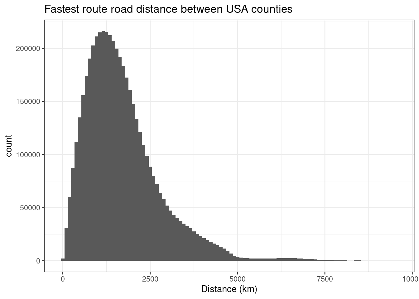
Distance information between places is useful to evaluate the proximity and interconnection of regions. The Euclidean distance between two places, although simple and easy to compute, is not realistic in terms of dislocation costs. This dataset present the road distance and trip duration metrics between all USA counties.

Methods

I used the county database from Simple Maps (basic 2024 version), with 3,144 entries.

A list of pairs of counties is computed using simple combinatorial analysis. Example:

x <- c("a", "b", "c", "d")

combn(x, m = 2)

     [,1] [,2] [,3] [,4] [,5] [,6]
[1,] "a"  "a"  "a"  "b"  "b"  "c" 
[2,] "b"  "c"  "d"  "c"  "d"  "d"

Note

With this, I assume that the distance between two counties is the same, independently of the direction.

Thus, for the 3,144 counties, we will have a total number of routes to be computed:

choose(n = 3144, k = 2)

[1] 4940796

To compute the road distance between pairs of counties, the OSRM API service was used, with the {osrm} package (Giraud 2022). More specifically, the table service was used, considering the “car” profile, returning as result the distance in meters and estimated trip duration in minutes for the fastest route found.

Route example

For example, lets compute the road distance between New York County, NY and Los Angeles Counties, CA with the {osrm} package.

library(osrm)
library(leaflet)
library(sf)

new_york <- c(-73.9668, 40.7792)
los_angeles <- c(-118.2247, 34.3219)

route <- osrmRoute(
  src = new_york, dst = los_angeles, 
  overview = "full",
  osrm.profile = "car"
)

# Route distance, in meters
route$distance

[1] 4516.204

# Route duration, in minutes
route$duration

[1] 2999.772

route |>
  st_transform(4326) |>
  leaflet() |>
  addTiles() |>
  addPolylines()

Important

For some pairs of municipalities, the OSRM service is not able to determine a possible road route. This is expected, as some municipalities are not reachable by road.

The scripts used to prepare the dataset are available here.

Dataset download

The dataset with the road distances and trip duration are available on Zenodo, on RDS format, parquet format, and CSV format.

Click the link below to access and download the data.

You can also download the dataset directly from R, using the {zendown} package.

# install.packages("zendown")
library(zendown)

dist_usa_file <- zen_file(13906981, "dist_usa.rds")

dist_usa <- readRDS(dist_usa_file)

head(dist_usa)

   orig  dest    dist    dur
1 06037 01073 3270056 2124.1
2 06037 01089 3251589 2136.9
3 06037 01097 3282597 2143.5
4 06037 04013  600220  412.8
5 06037 04019  823167  627.0
6 06037 04021  745854  524.8

Graphs

library(ggplot2)

ggplot(data = dist_usa, aes(x = dist/1000)) +
  geom_histogram(bins = 100) +
  labs(
    title = "Fastest route road distance between USA counties", 
    x = "Distance (km)", y = "count"
  ) +
  theme_bw()

ggplot(data = dist_usa, aes(x = dur/60)) +
  geom_histogram(bins = 100) +
  labs(
    title = "Fastest route estimated trip duration between USA counties", 
    x = "Trip duration (hours)", y = "count"
  ) +
  theme_bw()

Future plans

Compute routes using other available routing services.
Yearly updates of the dataset, as the road infrastructure may change.

References

Giraud, Timothée. 2022. “osrm: Interface Between R and the OpenStreetMap-Based Routing Service OSRM.” Journal of Open Source Software 7 (78): 4574. https://doi.org/10.21105/joss.04574.