Get started

The nseq package helps to count the number of sequences of values in a vector that meets conditions of length and magnitude.

As an example, let’s use the airquality dataset. It contains daily air quality measurements in New York, from May to September 1973.

library(nseq)
data("airquality")

head(airquality)
#>   Ozone Solar.R Wind Temp Month Day
#> 1    41     190  7.4   67     5   1
#> 2    36     118  8.0   72     5   2
#> 3    12     149 12.6   74     5   3
#> 4    18     313 11.5   62     5   4
#> 5    NA      NA 14.3   56     5   5
#> 6    28      NA 14.9   66     5   6

Examples

First, let’s consider the temperature measurements taken in June.

june_data <- subset(airquality, Month == 6)

library(ggplot2)

ggplot(june_data, aes(x = Day, y = Temp)) +
  geom_line() +
  geom_point() +
  theme_bw()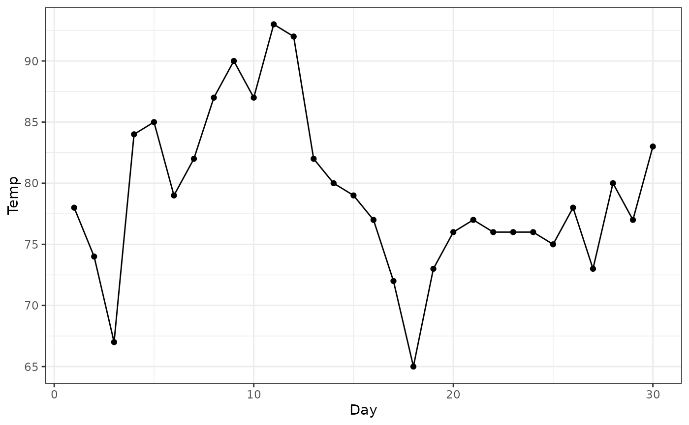

How many times we had three days or more in a row, with temperatures above 83F?

To answer this question, first look at the plot.

ggplot(june_data, aes(x = Day, y = Temp)) +
  geom_line() +
  geom_point() +
  geom_hline(yintercept = 83, color = "red") +
  theme_bw()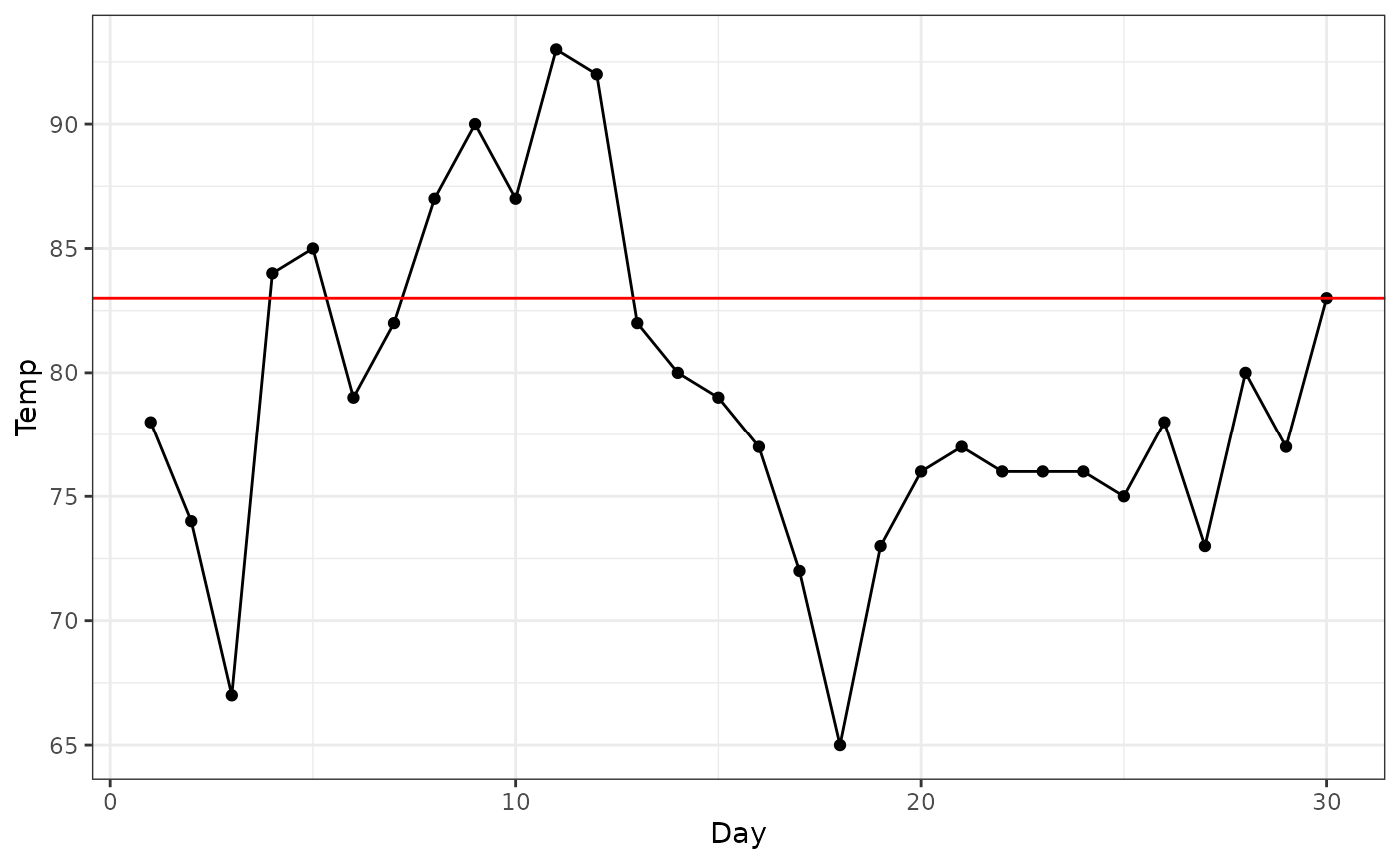

There are two sequences of days with temperatures above 83F. One with two days, and one with 5 days. This last sequence meets the condition of “three days or more”.

Now, let’s use the nseq package to compute this for us.

trle_cond(june_data$Temp, a_op = "gte", a = 3, b_op = "gte", b = 83)
#> [1] 1

How many times we had two days or more in sequence with temperatures below 75F?

ggplot(june_data, aes(x = Day, y = Temp)) +
  geom_line() +
  geom_point() +
  geom_hline(yintercept = 75, color = "red") +
  theme_bw()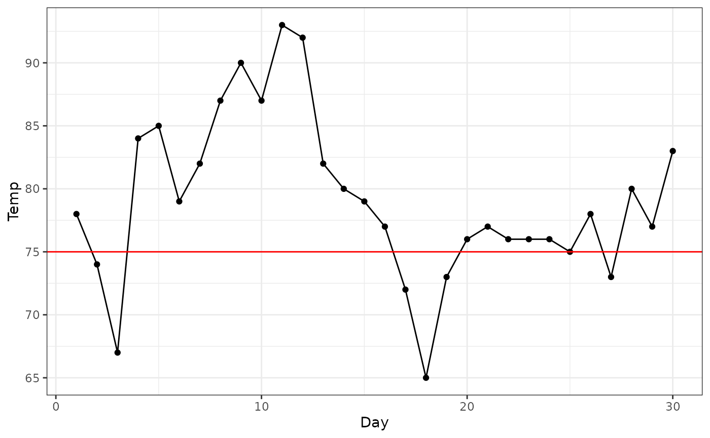

trle_cond(june_data$Temp, a_op = "gte", a = 2, b_op = "lte", b = 75)
#> [1] 2

Grouping

You can use the nseq functions inside ?dplyr::summarise to compute counts for groups.

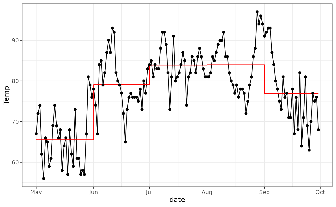
For each month, how many sequences of three days or more presented temperatures above the month’s average.

library(dplyr)

airquality |>
  summarise(
    avg = mean(Temp, na.rm = TRUE),
    count_3 = trle_cond(Temp, a_op = "gte", a = 3, b_op = "gte", b = avg), 
    .by = Month
  )
#>   Month      avg count_3
#> 1     5 65.54839       3
#> 2     6 79.10000       1
#> 3     7 83.90323       3
#> 4     8 83.96774       2
#> 5     9 76.90000       1

month_avg <- airquality |>
  summarise(
    avg = mean(Temp, na.rm = TRUE),
    .by = Month
  )

airquality |>
  left_join(month_avg, by = "Month") |>
  mutate(date = as.Date(paste0(1973,"-",Month,"-",Day))) |> 
  ggplot(aes(x = date)) +
    geom_line(aes(y = Temp)) +
    geom_step(aes(y = avg), color = "red") +
    geom_point(aes(y = Temp)) +
    theme_bw()