Para a leitura de arquivos shapefile no R, precisamos usar alguns pacotes. Após a instalação dos pacotes, use os seguintes comandos.
# Pacoteslibrary(sf)
Linking to GEOS 3.10.2, GDAL 3.4.1, PROJ 8.2.1; sf_use_s2() is TRUE
library(sp)
The legacy packages maptools, rgdal, and rgeos, underpinning the sp package,
which was just loaded, will retire in October 2023.
Please refer to R-spatial evolution reports for details, especially
https://r-spatial.org/r/2023/05/15/evolution4.html.
It may be desirable to make the sf package available;
package maintainers should consider adding sf to Suggests:.
The sp package is now running under evolution status 2
     (status 2 uses the sf package in place of rgdal)
# Abra o arquivo 'gm10.shp'fp_mg.shp <-st_read("data/FP_MG.shp", options ="ENCODING=WINDOWS-1252")
options:        ENCODING=WINDOWS-1252
Reading layer `FP_MG' from data source
  `/home/raphael/projects/ecoespacial/data/FP_MG.shp' using driver `ESRI Shapefile'
Warning in CPL_read_ogr(dsn, layer, query, as.character(options), quiet, : GDAL
Message 1: organizePolygons() received an unexpected geometry.  Either a
polygon with interior rings, or a polygon with less than 4 points, or a
non-Polygon geometry.  Return arguments as a collection.
Simple feature collection with 66 features and 41 fields
Geometry type: POLYGON
Dimension:     XY
Bounding box:  xmin: -51.06258 ymin: -22.91696 xmax: -39.85724 ymax: -14.23725
CRS:           NA
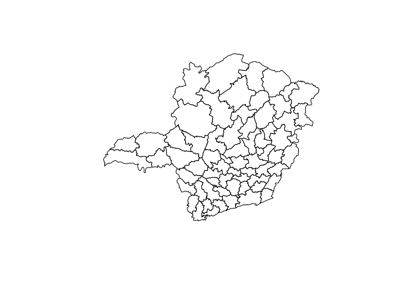
fp_mg.shp <-st_make_valid(fp_mg.shp)fp_mg.shp <-as_Spatial(fp_mg.shp)# encoding = "UTF-8"# Plotar o mapaplot(fp_mg.shp)
2.2 Atributos do shapefile
Podemos ver a tabela de atributos do shapefile desta forma.