5  Regressão Ponderada Geograficamente (GWR)

5.1 Pacote

library(mgwrsar)

Loading required package: Rcpp

Loading required package: sp

The legacy packages maptools, rgdal, and rgeos, underpinning the sp package,
which was just loaded, will retire in October 2023.
Please refer to R-spatial evolution reports for details, especially
https://r-spatial.org/r/2023/05/15/evolution4.html.
It may be desirable to make the sf package available;
package maintainers should consider adding sf to Suggests:.
The sp package is now running under evolution status 2
     (status 2 uses the sf package in place of rgdal)

Loading required package: leaflet

Loading required package: Matrix

5.2 Shapefile

# Pacotes
library(sf)

Linking to GEOS 3.10.2, GDAL 3.4.1, PROJ 8.2.1; sf_use_s2() is TRUE

library(sp)

# Abra o arquivo 'gm10.shp'
brmicro.shp <- st_read("data/br_micro.shp", options = "ENCODING=WINDOWS-1252")

options:        ENCODING=WINDOWS-1252 
Reading layer `br_micro' from data source 
  `/home/raphael/projects/ecoespacial/data/br_micro.shp' using driver `ESRI Shapefile'
Simple feature collection with 558 features and 5 fields
Geometry type: MULTIPOLYGON
Dimension:     XY
Bounding box:  xmin: -73.99095 ymin: -33.75086 xmax: -32.37889 ymax: 5.272225
CRS:           NA

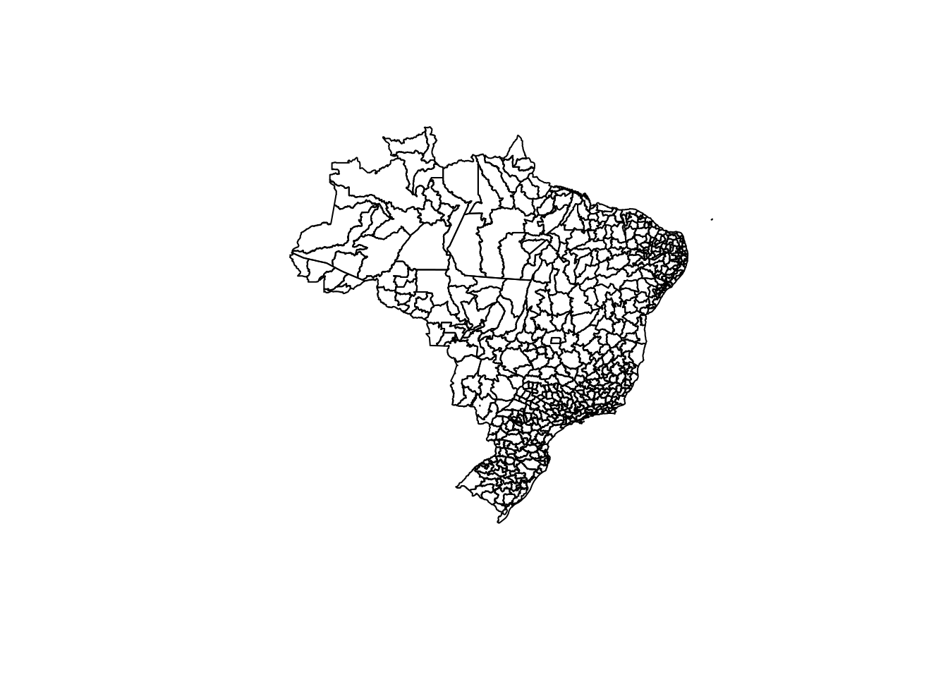
brmicro.shp <- st_make_valid(brmicro.shp)
brmicro.shp <- as_Spatial(brmicro.shp)

# Plotar o mapa
plot(brmicro.shp)

5.3 Dados

dados <- read.csv2("data/Dados_GWR.csv", header = TRUE)
str(dados)

'data.frame':   558 obs. of  17 variables:
 $ ID     : int  110001 110002 110003 110004 110005 110006 110007 110008 120001 120002 ...
 $ X_COORD: num  -64.5 -63.8 -62.6 -62.5 -62.8 ...
 $ Y_COORD: num  -9.42 -11.68 -9.53 -10.54 -11.67 ...
 $ P9303  : num  -0.0492 0.0584 0.2066 0.0747 0.157 ...
 $ Q9303  : num  0.881 0.148 0.195 -0.627 0.366 ...
 $ P93    : num  8.3 4.64 2.54 3.1 1.82 ...
 $ G0     : num  0 0.44 0.694 0.626 0.781 ...
 $ CT9303 : num  1.91 1.71 1.66 2.21 3.08 ...
 $ CI9303 : num  1.147 2.03 -1.385 -0.294 1.647 ...
 $ CC9303 : num  1.206 -0.165 1.662 1.975 2.734 ...
 $ WP9303 : num  0.2632 0.0802 0.1186 0.0738 0.0905 ...
 $ WQ9303 : num  0.853 0.146 1.075 0.42 -0.171 ...
 $ WP93   : num  3.79 3.54 3.96 2.65 2.89 ...
 $ WG0    : num  0.409 0.544 0.372 0.546 0.612 ...
 $ WCT9303: num  1.62 2.49 1.15 2.08 2.23 ...
 $ WCI9303: num  -0.817 0.809 0.718 1.654 0.824 ...
 $ WCC9303: num  1.64 2.09 1.02 1.33 1.42 ...

5.4 Especificação

Q9303 : Taxa de crescimento da produção agrícola microrregional no período de 1993 a 2003

P9303: Taxa de crescimento da produtividade da terra no período de 1993 a 2003

G0: medida de gap tecnológico

CI9303: taxa de crescimento do crédito para investimento agrícola no período de 1993 a 2003.

esp <- Q9303 ~ P9303 + G0 + CI9303

5.5 Modelo OLS

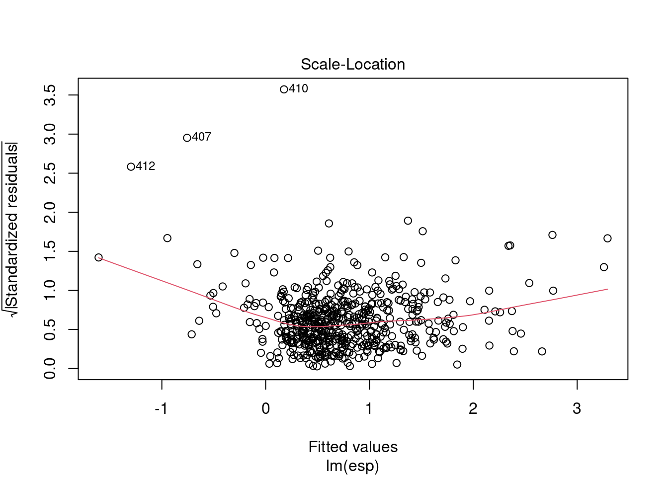
mod1 <- lm(formula = esp, data = dados)
summary(mod1)

Call:
lm(formula = esp, data = dados)

Residuals:
    Min      1Q  Median      3Q     Max 
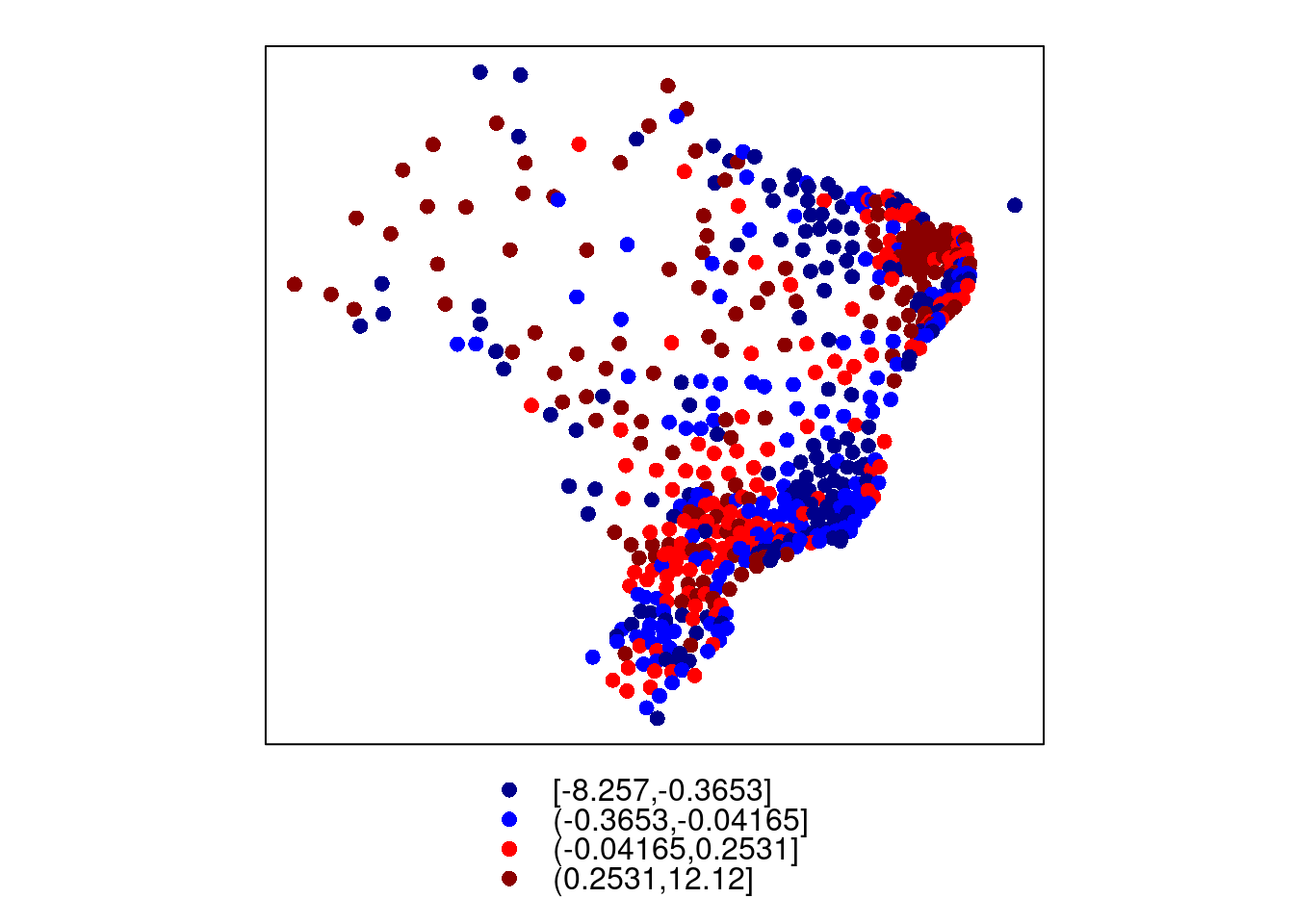
-8.2571 -0.3653 -0.0417  0.2531 12.1204 

Coefficients:
             Estimate Std. Error t value Pr(>|t|)    
(Intercept)  0.255015   0.054681   4.664  3.9e-06 ***
P9303        1.692115   0.124878  13.550  < 2e-16 ***
G0           0.041733   0.033751   1.236    0.217    
CI9303      -0.002689   0.019658  -0.137    0.891    
---
Signif. codes:  0 '***' 0.001 '**' 0.01 '*' 0.05 '.' 0.1 ' ' 1

Residual standard error: 0.9564 on 554 degrees of freedom
Multiple R-squared:  0.2672,    Adjusted R-squared:  0.2632 
F-statistic: 67.33 on 3 and 554 DF,  p-value: < 2.2e-16

5.6 Verificando erros do modelo

plot(mod1, which=3)

5.7 Verificando resíduos no espaço

resids <- residuals(mod1)
cores <- c("dark blue", "blue", "red", "dark red") 
map.resids <- SpatialPointsDataFrame(data=data.frame(resids), coords=cbind(dados$X_COORD,dados$Y_COORD)) 
spplot(map.resids, cuts=quantile(resids), col.regions=cores, cex=1) 

5.8 GWR com kernel gaussiano

coord <- as.matrix(cbind(dados$X_COORD,dados$Y_COORD))

mod1.gwr <- MGWRSAR(formula = esp, data = dados, 
                    coord = coord,
                    fixed_vars = NULL, kernels = c('gauss'), H = 0.60,
                    Model = 'GWR',
                    control=list(SE = TRUE, doMC = TRUE, ncore = 4))

summary_mgwrsar(mod1.gwr)

Call:
MGWRSAR(formula = esp, data = dados, coord = coord, fixed_vars = NULL, 
    kernels = c("gauss"), H = 0.6, Model = "GWR", control = list(SE = TRUE, 
        doMC = TRUE, ncore = 4))
Model: GWR 
Kernels function: gauss 
Kernels adaptive: NO 
Kernels type: GD 
Bandwidth: 0.6 
Computation time: 0.821 
Use of parallel computing: TRUE  ncore = 4 
Use of rough kernel: NO 
Use of Target Points: NO 
Number of data points: 558 
Varying parameters: Intercept P9303 G0 CI9303 
          Intercept       P9303          G0  CI9303
Min.    -8.2811e+02 -2.1688e+01 -7.6471e+00 -2.6374
1st Qu. -1.9185e-01  9.8576e-01 -2.7433e-01 -0.0609
Median   1.1666e-01  1.8369e+00 -1.5489e-03  0.0025
Mean    -1.9452e+00  1.8003e+00  2.1188e+00  0.0377
3rd Qu.  5.2344e-01  2.3682e+00  3.2038e-01  0.0652
Max.     6.2005e+00  3.3002e+01  8.3419e+02  2.1745
Effective degrees of freedom: 214.4194 
AIC 1286.154 
Residual sum of squares: 176.9171 
RMSE: 0.5630771 

plot_mgwrsar(mod1.gwr,type='B_coef',var='CI9303', radius = 20000)

plot_mgwrsar(mod1.gwr,type='t_coef',var='CI9303', radius = 20000)

5.9 GWR com ‘CV leave one out’ e kernel adaptativo biquadrado (considerando 20 vizinhos) e remoção de outliers

mod2.gwr <- MGWRSAR(formula = esp, data = dados, coord=coord,
                    fixed_vars = NULL, kernels = c('bisq'), H=20,
                    Model = 'GWR',
                    control=list(isgcv=TRUE,remove_local_outlier=TRUE,outv=0.01))
summary_mgwrsar(mod2.gwr)

Call:
MGWRSAR(formula = esp, data = dados, coord = coord, fixed_vars = NULL, 
    kernels = c("bisq"), H = 20, Model = "GWR", control = list(isgcv = TRUE, 
        remove_local_outlier = TRUE, outv = 0.01))
Model: GWR 
Kernels function: bisq 
Kernels adaptive: NO 
Kernels type: GD 
Bandwidth: 20 
Computation time: 0.636 
Use of parallel computing: FALSE  ncore = 1 
Use of rough kernel: NO 
Use of Target Points: NO 
Number of data points: 558 
Varying parameters: Intercept P9303 G0 CI9303 
          Intercept       P9303          G0  CI9303
Min.     0.10424379  0.90006692 -1.34446628 -0.1101
1st Qu.  0.15206433  1.67545203  0.00461598 -0.0202
Median   0.21499269  1.70988054  0.02319197 -0.0138
Mean     0.24363087  1.71237373  0.00073565 -0.0121
3rd Qu.  0.27568400  1.77191031  0.08011017 -0.0071
Max.     1.23604439  2.16398074  0.10863633  0.0588
Residual sum of squares: 499.5637 
RMSE: 0.94619 

plot_mgwrsar(mod2.gwr, type='B_coef',var='G0', radius = 20000)

Saiba mais em: https://cran.r-project.org/web/packages/mgwrsar/vignettes/mgwrsar-basic_examples.html

5.10 Usando o pacote spgwr

library(spgwr)

Loading required package: spData

To access larger datasets in this package, install the spDataLarge
package with: `install.packages('spDataLarge',
repos='https://nowosad.github.io/drat/', type='source')`

NOTE: This package does not constitute approval of GWR
as a method of spatial analysis; see example(gwr)

5.10.1 Kernel bandwith

GWRbandwidth <- gwr.sel(esp, data=dados, coords = cbind(dados$X_COORD,dados$Y_COORD), adapt = TRUE) 

Adaptive q: 0.381966 CV score: 513.9403 
Adaptive q: 0.618034 CV score: 514.5733 
Adaptive q: 0.236068 CV score: 510.1655 
Adaptive q: 0.145898 CV score: 509.9981 
Adaptive q: 0.1818601 CV score: 509.6378 
Adaptive q: 0.1867464 CV score: 509.5685 
Adaptive q: 0.2055856 CV score: 509.9121 
Adaptive q: 0.1894925 CV score: 509.6879 
Adaptive q: 0.1852418 CV score: 509.6098 
Adaptive q: 0.1877954 CV score: 509.6292 
Adaptive q: 0.1864049 CV score: 509.5482 
Adaptive q: 0.1861779 CV score: 509.5577 
Adaptive q: 0.1864456 CV score: 509.5506 
Adaptive q: 0.1863466 CV score: 509.5485 
Adaptive q: 0.1864049 CV score: 509.5482 

5.10.2 Modelo GWR

mod4.gwr = gwr(esp, data=dados, coords = cbind(dados$X_COORD,dados$Y_COORD), adapt=GWRbandwidth, hatmatrix=TRUE, se.fit=TRUE) 
mod4.gwr

Call:
gwr(formula = esp, data = dados, coords = cbind(dados$X_COORD, 
    dados$Y_COORD), adapt = GWRbandwidth, hatmatrix = TRUE, se.fit = TRUE)
Kernel function: gwr.Gauss 
Adaptive quantile: 0.1864049 (about 104 of 558 data points)
Summary of GWR coefficient estimates at data points:
                  Min.   1st Qu.    Median   3rd Qu.      Max.  Global
X.Intercept. -0.276464 -0.066091  0.143081  0.367378  0.612604  0.2550
P9303         1.207676  1.483514  1.872278  2.474311  2.747145  1.6921
G0           -0.081195 -0.034559  0.015841  0.118441  0.173140  0.0417
CI9303       -0.046286 -0.028744  0.016651  0.074686  0.121517 -0.0027
Number of data points: 558 
Effective number of parameters (residual: 2traceS - traceS'S): 17.35644 
Effective degrees of freedom (residual: 2traceS - traceS'S): 540.6436 
Sigma (residual: 2traceS - traceS'S): 0.9203189 
Effective number of parameters (model: traceS): 13.31951 
Effective degrees of freedom (model: traceS): 544.6805 
Sigma (model: traceS): 0.9169021 
Sigma (ML): 0.9058927 
AICc (GWR p. 61, eq 2.33; p. 96, eq. 4.21): 1502.684 
AIC (GWR p. 96, eq. 4.22): 1486.556 
Residual sum of squares: 457.918 
Quasi-global R2: 0.3378047