Para a leitura de arquivos shapefile no R, precisamos usar alguns pacotes. Após a instalação dos pacotes, use os seguintes comandos.
# Pacoteslibrary(sf)
Linking to GEOS 3.10.2, GDAL 3.4.1, PROJ 8.2.1; sf_use_s2() is TRUE
library(sp)
The legacy packages maptools, rgdal, and rgeos, underpinning the sp package,
which was just loaded, will retire in October 2023.
Please refer to R-spatial evolution reports for details, especially
https://r-spatial.org/r/2023/05/15/evolution4.html.
It may be desirable to make the sf package available;
package maintainers should consider adding sf to Suggests:.
The sp package is now running under evolution status 2
     (status 2 uses the sf package in place of rgdal)
# Abra o arquivo 'gm10.shp'fp_mg.shp <-st_read("data/FP_MG.shp", options ="ENCODING=WINDOWS-1252")
options:        ENCODING=WINDOWS-1252
Reading layer `FP_MG' from data source
  `/home/raphael/projects/ecoespacial/data/FP_MG.shp' using driver `ESRI Shapefile'
Warning in CPL_read_ogr(dsn, layer, query, as.character(options), quiet, : GDAL
Message 1: organizePolygons() received an unexpected geometry.  Either a
polygon with interior rings, or a polygon with less than 4 points, or a
non-Polygon geometry.  Return arguments as a collection.
Simple feature collection with 66 features and 41 fields
Geometry type: POLYGON
Dimension:     XY
Bounding box:  xmin: -51.06258 ymin: -22.91696 xmax: -39.85724 ymax: -14.23725
CRS:           NA
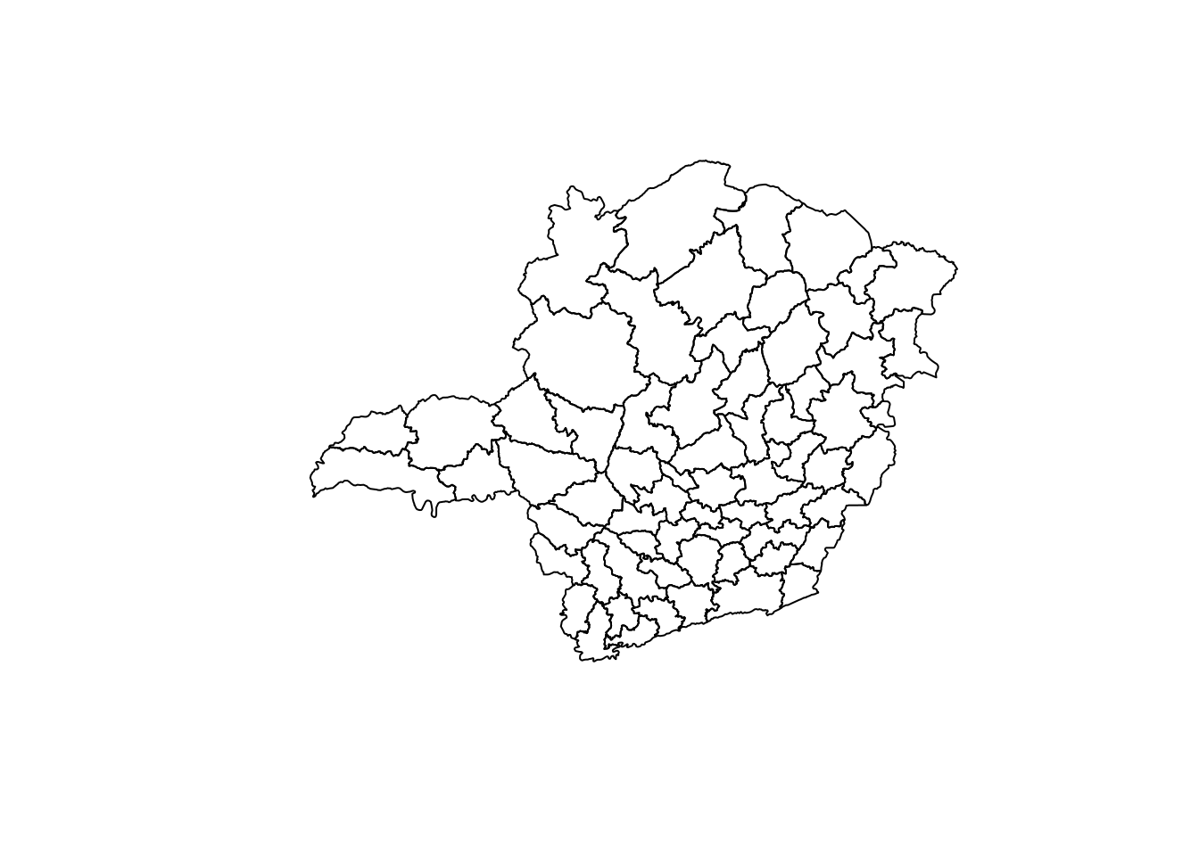
fp_mg.shp <-st_make_valid(fp_mg.shp)fp_mg.shp <-as_Spatial(fp_mg.shp)# Plotar o mapaplot(fp_mg.shp)
Para a criação de matrizes de vizinhos espaciais, iremos utilizar o pacote spdep.
# Pacotelibrary(spdep)
Loading required package: spData
To access larger datasets in this package, install the spDataLarge
package with: `install.packages('spDataLarge',
repos='https://nowosad.github.io/drat/', type='source')`
Characteristics of weights list object:
Neighbour list object:
Number of regions: 66
Number of nonzero links: 336
Percentage nonzero weights: 7.713499
Average number of links: 5.090909
Link number distribution:

 2  3  4  5  6  7  8  9
 2  9 12 16 16  8  2  1
2 least connected regions:
29 38 with 2 links
1 most connected region:
65 with 9 links

Weights style: W
Weights constants summary:
   n   nn S0       S1       S2
W 66 4356 66 27.58858 269.8006
# Matriz queen 2ª ordemw1.2<-nb2listw(nblag_cumul(nblag(poly2nb(fp_mg.shp, queen =TRUE), maxlag =2)))# Matrix queen padronizada na linhaw1.w <-nb2listw(poly2nb(fp_mg.shp, queen=TRUE), style="W")summary(w1.w)
Characteristics of weights list object:
Neighbour list object:
Number of regions: 66
Number of nonzero links: 336
Percentage nonzero weights: 7.713499
Average number of links: 5.090909
Link number distribution:

 2  3  4  5  6  7  8  9
 2  9 12 16 16  8  2  1
2 least connected regions:
29 38 with 2 links
1 most connected region:
65 with 9 links

Weights style: W
Weights constants summary:
   n   nn S0       S1       S2
W 66 4356 66 27.58858 269.8006
Characteristics of weights list object:
Neighbour list object:
Number of regions: 66
Number of nonzero links: 332
Percentage nonzero weights: 7.621671
Average number of links: 5.030303
Link number distribution:

 2  3  4  5  6  7  8
 2  9 12 18 15  7  3
2 least connected regions:
29 38 with 2 links
3 most connected regions:
12 26 65 with 8 links

Weights style: W
Weights constants summary:
   n   nn S0       S1       S2
W 66 4356 66 27.82221 269.6778
Characteristics of weights list object:
Neighbour list object:
Number of regions: 66
Number of nonzero links: 332
Percentage nonzero weights: 7.621671
Average number of links: 5.030303
Link number distribution:

 2  3  4  5  6  7  8
 2  9 12 18 15  7  3
2 least connected regions:
29 38 with 2 links
3 most connected regions:
12 26 65 with 8 links

Weights style: C
Weights constants summary:
   n   nn S0       S1      S2
C 66 4356 66 26.24096 285.489
Characteristics of weights list object:
Neighbour list object:
Number of regions: 66
Number of nonzero links: 4290
Percentage nonzero weights: 98.48485
Average number of links: 65
Link number distribution:

65
66
66 least connected regions:
1 2 3 4 5 6 7 8 9 10 11 12 13 14 15 16 17 18 19 20 21 22 23 24 25 26 27 28 29 30 31 32 33 34 35 36 37 38 39 40 41 42 43 44 45 46 47 48 49 50 51 52 53 54 55 56 57 58 59 60 61 62 63 64 65 66 with 65 links
66 most connected regions:
1 2 3 4 5 6 7 8 9 10 11 12 13 14 15 16 17 18 19 20 21 22 23 24 25 26 27 28 29 30 31 32 33 34 35 36 37 38 39 40 41 42 43 44 45 46 47 48 49 50 51 52 53 54 55 56 57 58 59 60 61 62 63 64 65 66 with 65 links

Weights style: W
Weights constants summary:
   n   nn S0       S1       S2
W 66 4356 66 8.369751 267.6908
# Distância inversa padronizada pelo número de vizinhosw3.u <-nb2listw(nb, glist=dlist, style="U")summary(w3.u)
Characteristics of weights list object:
Neighbour list object:
Number of regions: 66
Number of nonzero links: 4290
Percentage nonzero weights: 98.48485
Average number of links: 65
Link number distribution:

65
66
66 least connected regions:
1 2 3 4 5 6 7 8 9 10 11 12 13 14 15 16 17 18 19 20 21 22 23 24 25 26 27 28 29 30 31 32 33 34 35 36 37 38 39 40 41 42 43 44 45 46 47 48 49 50 51 52 53 54 55 56 57 58 59 60 61 62 63 64 65 66 with 65 links
66 most connected regions:
1 2 3 4 5 6 7 8 9 10 11 12 13 14 15 16 17 18 19 20 21 22 23 24 25 26 27 28 29 30 31 32 33 34 35 36 37 38 39 40 41 42 43 44 45 46 47 48 49 50 51 52 53 54 55 56 57 58 59 60 61 62 63 64 65 66 with 65 links

Weights style: U
Weights constants summary:
   n   nn S0          S1         S2
U 66 4356  1 0.002368187 0.07316268
Para ver mais opções, veja a ajuda deste comando: ?nb2listw
3.1.3 Matriz de k-vizinhos espaciais
A escolha do número ideal de \(k\) vizinhos será realizada testando-se vários \(k\) e utilizando-se o que retornou o maior valor para a estatística \(I\) de Moran significativo.
# Número de permutaçõesper <-999# Número máximo de k vizinhos testadoskv <-20# Nome dos registrosIDs <-row.names(fp_mg.shp@data)# Criação da tabela que irá receber a estatística I de Moran e significância para cada k testadores.pesos <-data.frame(k=numeric(),i=numeric(),valorp=numeric())# Início do loopfor(k in1:kv){# Armazenando número k atual res.pesos[k,1] <- k# Calculando o I e significância para o k atual moran.k <-moran.mc(fp_mg.shp@data$Q,listw=nb2listw(knn2nb(knearneigh(coords, k=k),row.names=IDs),style="B"),nsim=per)# Armazenando o valor I para o k atual res.pesos[k,2] <- moran.k$statistic# Armazenando o p-value para o k atual res.pesos[k,3] <- moran.k$p.value}# Ver a tabela de k vizinhos, I de Moran e significânciares.pesos
# Sendo todos significativos, iremos usar o k que retornou o maior valor Imaxi <-which.max(res.pesos[,2])# Criação da matriz usando o k escolhidow5 <-nb2listw(knn2nb(knearneigh(coords, k=maxi),row.names=IDs),style="B")summary(w5)
Characteristics of weights list object:
Neighbour list object:
Number of regions: 66
Number of nonzero links: 66
Percentage nonzero weights: 1.515152
Average number of links: 1
Non-symmetric neighbours list
Link number distribution:

 1
66
66 least connected regions:
1 2 3 4 5 6 7 8 9 10 11 12 13 14 15 16 17 18 19 20 21 22 23 24 25 26 27 28 29 30 31 32 33 34 35 36 37 38 39 40 41 42 43 44 45 46 47 48 49 50 51 52 53 54 55 56 57 58 59 60 61 62 63 64 65 66 with 1 link
66 most connected regions:
1 2 3 4 5 6 7 8 9 10 11 12 13 14 15 16 17 18 19 20 21 22 23 24 25 26 27 28 29 30 31 32 33 34 35 36 37 38 39 40 41 42 43 44 45 46 47 48 49 50 51 52 53 54 55 56 57 58 59 60 61 62 63 64 65 66 with 1 link

Weights style: B
Weights constants summary:
   n   nn S0 S1  S2
B 66 4356 66 98 308
3.2 Autocorrelação espacial global
3.2.1 I de Moran
moran.test(fp_mg.shp@data$Q, listw = w5)
    Moran I test under randomisation

data:  fp_mg.shp@data$Q
weights: w5

Moran I statistic standard deviate = 3.8645, p-value = 5.566e-05
alternative hypothesis: greater
sample estimates:
Moran I statistic       Expectation          Variance
       0.52280745       -0.01538462        0.01939499
moran.mc(fp_mg.shp@data$Q, listw = w5, nsim =999)
    Monte-Carlo simulation of Moran I

data:  fp_mg.shp@data$Q
weights: w5
number of simulations + 1: 1000

statistic = 0.52281, observed rank = 997, p-value = 0.003
alternative hypothesis: greater
3.2.2 C de Geary
geary.test(fp_mg.shp@data$Q, listw = w5)
    Geary C test under randomisation

data:  fp_mg.shp@data$Q
weights: w5

Geary C statistic standard deviate = 2.6176, p-value = 0.004428
alternative hypothesis: Expectation greater than statistic
sample estimates:
Geary C statistic       Expectation          Variance
       0.46130049        1.00000000        0.04235442
geary.mc(fp_mg.shp@data$Q, listw = w5, nsim =999)
    Monte-Carlo simulation of Geary C

data:  fp_mg.shp@data$Q
weights: w5
number of simulations + 1: 1000

statistic = 0.4613, observed rank = 5, p-value = 0.005
alternative hypothesis: greater
3.2.3 G de Getis-Ord
globalG.test(as.vector(scale(fp_mg.shp@data$Q, center =FALSE)), listw = w5, B1correct =TRUE)
    Getis-Ord global G statistic

data:  as.vector(scale(fp_mg.shp@data$Q, center = FALSE))
weights: w5

standard deviate = 3.2113, p-value = 0.0006607
alternative hypothesis: greater
sample estimates:
Global G statistic        Expectation           Variance
      3.071155e-02       1.538462e-02       2.277991e-05
       Ii                E.Ii                Var.Ii               Z.Ii
 Min.   :-0.83956   Min.   :-2.629e-01   Min.   : 0.000197   Min.   :-4.1007
 1st Qu.: 0.07066   1st Qu.:-4.908e-03   1st Qu.: 0.089934   1st Qu.: 0.2869
 Median : 0.20075   Median :-3.384e-03   Median : 0.222559   Median : 0.4695
 Mean   : 0.52281   Mean   :-1.538e-02   Mean   : 0.860585   Mean   : 0.3957
 3rd Qu.: 0.27959   3rd Qu.:-1.365e-03   3rd Qu.: 0.322327   3rd Qu.: 0.5559
 Max.   :11.31579   Max.   :-2.980e-06   Max.   :12.789972   Max.   : 4.2162
 Pr(z != E(Ii))
 Min.   :0.0000248
 1st Qu.:0.5703228
 Median :0.6347460
 Mean   :0.6120352
 3rd Qu.:0.7541930
 Max.   :0.9892306
# Quantos são significativos?lm1 <-as.data.frame(lm1)table(lm1$`Pr(z != E(Ii))`<0.05)
FALSE  TRUE
   61     5
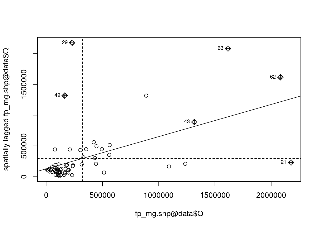
3.4 Diagrama de dispersão de Moran
moran.plot(fp_mg.shp@data$Q, listw = w5)
3.4.1 Sua vez
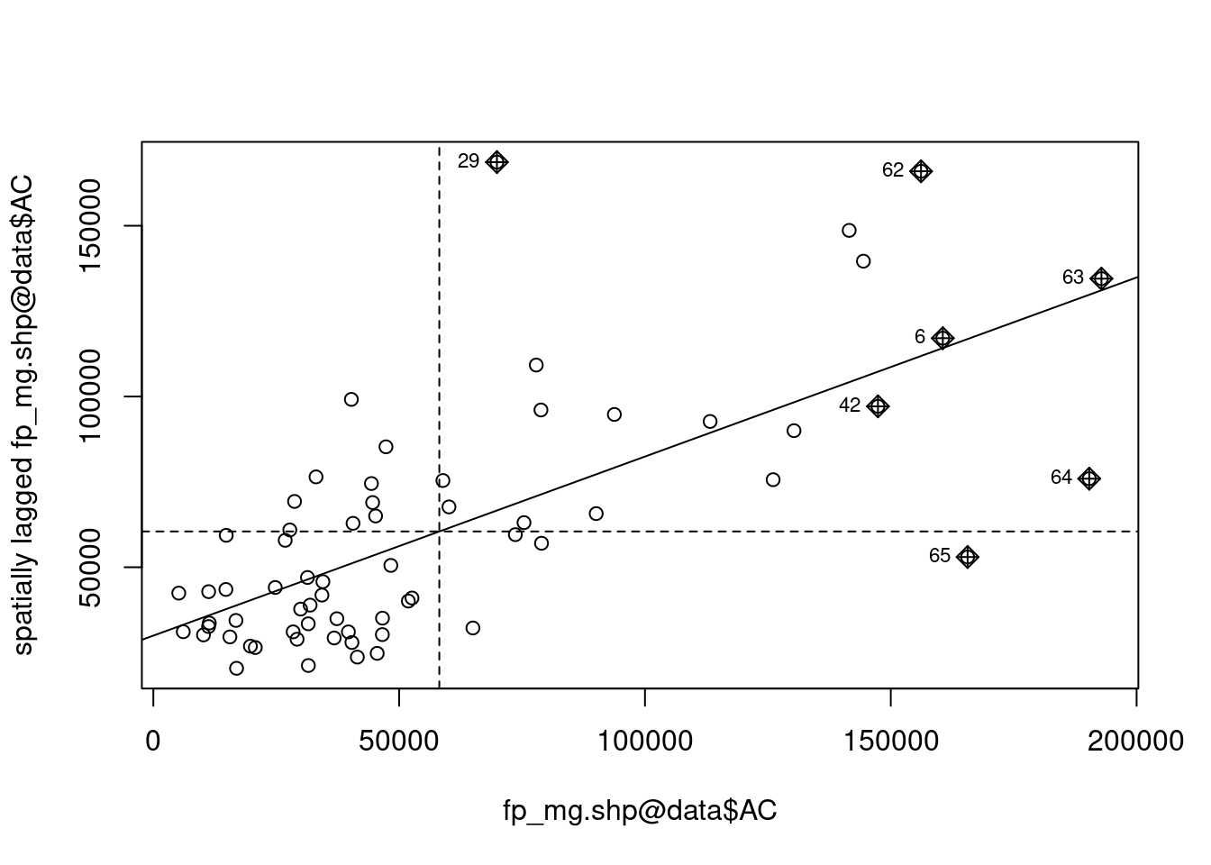
Calcule o I de Moran local usando a matriz de vizinhança w1 para a variável ACe verifique quantas regiões são significativas. Depois, faça o diagrama de dispersão.
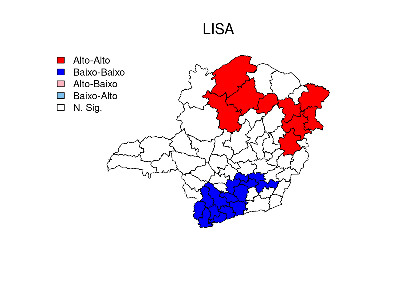
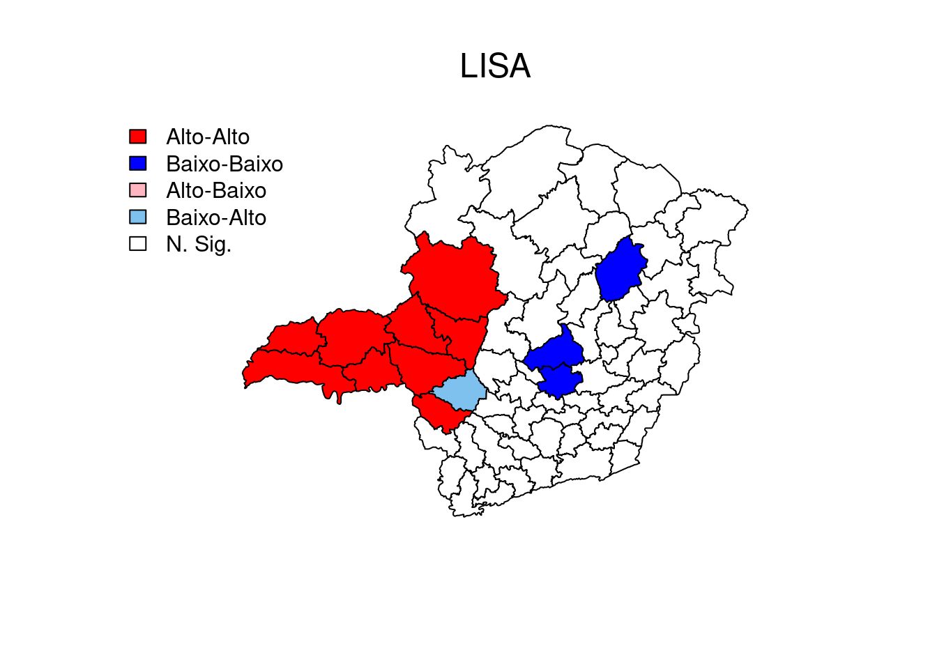
O R não tem uma função pronta para criar um mapa LISA, então nós criamos abaixo nossa própria função: lisaplot. Depois de declarada, uma função pode ser usada repetidamente variando seus argumentos.