6  Modelos espaciais em painel

6.1 Pacotes

O pacote plm é responsável pelos painéis convencionais (não espaciais) que usaremos para comparação. O pacote splm é responsável pelos painéis espaciais. Os autores do pacote lançaram um artigo sobre ele neste link.

library(spatialreg)
Loading required package: spData
The legacy packages maptools, rgdal, and rgeos, underpinning the sp package,
which was just loaded, will retire in October 2023.
Please refer to R-spatial evolution reports for details, especially
https://r-spatial.org/r/2023/05/15/evolution4.html.
It may be desirable to make the sf package available;
package maintainers should consider adding sf to Suggests:.
The sp package is now running under evolution status 2
     (status 2 uses the sf package in place of rgdal)
To access larger datasets in this package, install the spDataLarge
package with: `install.packages('spDataLarge',
repos='https://nowosad.github.io/drat/', type='source')`
Loading required package: Matrix
Loading required package: sf
Linking to GEOS 3.10.2, GDAL 3.4.1, PROJ 8.2.1; sf_use_s2() is TRUE
library(plm)
library(splm)

Attaching package: 'splm'
The following object is masked from 'package:spatialreg':

    impacts

6.2 Shapefile

# Pacotes
library(sf)
library(sp)

# Abra o arquivo
natregimes_montana.shp <- st_read("data/natregimes_montana.gml")
Reading layer `natregimes_montana' from data source 
  `/home/raphael/projects/ecoespacial/data/natregimes_montana.gml' 
  using driver `GML'
Simple feature collection with 55 features and 74 fields
Geometry type: MULTIPOLYGON
Dimension:     XY
Bounding box:  xmin: -116.0625 ymin: 44.35373 xmax: -104.0426 ymax: 49
Geodetic CRS:  WGS 84
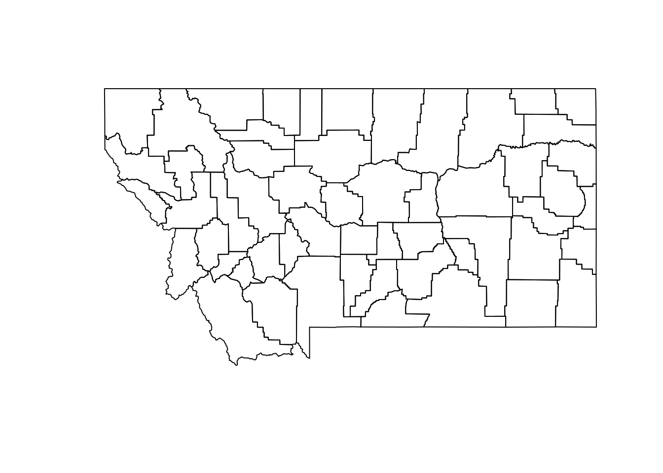
natregimes_montana.shp <- st_make_valid(natregimes_montana.shp)
natregimes_montana.shp <- as_Spatial(natregimes_montana.shp)

# Plotar o mapa
plot(natregimes_montana.shp)

6.3 Dados

Uma olhada nos dados.

str(natregimes_montana.shp@data)
'data.frame':   55 obs. of  74 variables:
 $ fid       : chr  "natregimes_montana.0" "natregimes_montana.1" "natregimes_montana.2" "natregimes_montana.3" ...
 $ REGIONS   : num  2 2 2 2 2 2 2 2 2 2 ...
 $ NOSOUTH   : num  1 1 1 1 1 1 1 1 1 1 ...
 $ POLY_ID   : int  7 8 9 10 11 12 13 24 25 26 ...
 $ NAME      : chr  "Lincoln" "Flathead" "Glacier" "Toole" ...
 $ STATE_NAME: chr  "Montana" "Montana" "Montana" "Montana" ...
 $ STATE_FIPS: int  30 30 30 30 30 30 30 30 30 30 ...
 $ CNTY_FIPS : int  53 29 35 101 51 41 91 5 71 105 ...
 $ FIPS      : int  30053 30029 30035 30101 30051 30041 30091 30005 30071 30105 ...
 $ STFIPS    : int  30 30 30 30 30 30 30 30 30 30 ...
 $ COFIPS    : int  53 29 35 101 51 41 91 5 71 105 ...
 $ FIPSNO    : int  30053 30029 30035 30101 30051 30041 30091 30005 30071 30105 ...
 $ SOUTH     : int  0 0 0 0 0 0 0 0 0 0 ...
 $ HR60      : num  7.98 1.01 11.53 0 0 ...
 $ HR70      : num  5.54 1.69 9.27 5.71 0 ...
 $ HR80      : num  5.63 4.49 28.23 0 0 ...
 $ HR90      : num  5.72 2.81 5.5 6.61 0 ...
 $ HC60      : num  1 0.333 1.333 0 0 ...
 $ HC70      : num  1 0.667 1 0.333 0 ...
 $ HC80      : num  1 2.33 3 0 0 ...
 $ HC90      : num  1 1.667 0.667 0.333 0 ...
 $ PO60      : int  12537 32965 11565 7904 2624 18653 6458 8091 6027 17080 ...
 $ PO70      : int  18063 39460 10783 5839 2359 17358 5779 6727 5386 11471 ...
 $ PO80      : int  17752 51966 10628 5559 2329 17985 5414 6999 5367 10250 ...
 $ PO90      : int  17481 59218 12121 5046 2295 17654 4732 6728 5163 8239 ...
 $ RD60      : num  -1.404 -1.136 -0.315 -1.246 -0.972 ...
 $ RD70      : num  -1.543 -0.885 0.201 -0.636 -0.73 ...
 $ RD80      : num  -0.907 -0.939 0.413 -0.314 -0.181 ...
 $ RD90      : num  -0.234 -0.305 1.479 -0.649 -0.298 ...
 $ PS60      : num  -0.982 -0.346 -0.967 -1.117 -1.865 ...
 $ PS70      : num  -0.698 -0.232 -1.002 -1.314 -1.878 ...
 $ PS80      : num  -0.797 -0.131 -1.107 -1.433 -1.965 ...
 $ PS90      : num  -0.8041 -0.0598 -1.0004 -1.4703 -1.9292 ...
 $ UE60      : num  17.3 13.8 12.8 5.5 5.1 6.3 5.5 7.1 4.3 8.6 ...
 $ UE70      : num  10.3 9.8 12.6 3.6 0.5 4.3 3 10.6 4.3 5.1 ...
 $ UE80      : num  27.53 14.23 8.56 3.55 1.83 ...
 $ UE90      : num  16.12 7.72 16.96 1.85 2.6 ...
 $ DV60      : num  3.44 2.6 3.86 3.3 2.4 ...
 $ DV70      : num  3.8 3.3 3.5 4.07 3.11 ...
 $ DV80      : num  6.13 6.22 5.84 4.64 4.21 ...
 $ DV90      : num  9.57 9.28 7.82 7.69 4.44 ...
 $ MA60      : num  24.8 30.1 22.8 25.9 24.8 24 29.2 25.3 28.9 23.4 ...
 $ MA70      : num  25.1 28 22.1 29.4 26.9 24.2 31.3 26.8 29 25.2 ...
 $ MA80      : num  28.3 29.7 26.8 29.9 30 27.2 33.4 27.5 29.6 29.4 ...
 $ MA90      : num  34.7 35.3 28.2 35.3 34 31.7 39.6 31.6 34 36.9 ...
 $ POL60     : num  9.44 10.4 9.36 8.98 7.87 ...
 $ POL70     : num  9.8 10.58 9.29 8.67 7.77 ...
 $ POL80     : num  9.78 10.86 9.27 8.62 7.75 ...
 $ POL90     : num  9.77 10.99 9.4 8.53 7.74 ...
 $ DNL60     : num  1.217 1.859 1.361 1.4 0.601 ...
 $ DNL70     : num  1.582 2.039 1.291 1.097 0.494 ...
 $ DNL80     : num  1.59 2.32 1.27 1.06 0.49 ...
 $ DNL90     : num  1.577 2.452 1.398 0.971 0.473 ...
 $ MFIL59    : num  8.61 8.59 8.55 8.7 8.68 ...
 $ MFIL69    : num  9.18 9.06 8.94 9.05 9.06 ...
 $ MFIL79    : num  9.77 9.83 9.66 9.76 9.76 ...
 $ MFIL89    : num  10.13 10.26 9.98 10.3 10.24 ...
 $ FP59      : num  16.8 20 28.7 12.7 16 14.7 27.9 30.8 30.6 21.1 ...
 $ FP69      : num  5.9 10.1 23.4 10.9 8.1 11.1 8.2 25.2 13.1 14 ...
 $ FP79      : num  9.55 6.91 16.72 9.4 14.15 ...
 $ FP89      : num  11.7 11.7 30.5 10 11.9 ...
 $ BLK60     : num  0.0239 0.0819 0.2075 0.0127 0 ...
 $ BLK70     : num  0.0221 0.076 0.0278 0 0 ...
 $ BLK80     : num  0.0394 0.0712 0.0282 0.018 0 ...
 $ BLK90     : num  0.0629 0.0946 0.0908 0.0991 0.1307 ...
 $ GI59      : num  0.211 0.242 0.317 0.24 0.286 ...
 $ GI69      : num  0.296 0.335 0.381 0.355 0.379 ...
 $ GI79      : num  0.312 0.336 0.382 0.38 0.391 ...
 $ GI89      : num  0.367 0.373 0.428 0.344 0.378 ...
 $ FH60      : num  6.87 7.86 12.64 9.44 9.23 ...
 $ FH70      : num  3.7 6.4 11.4 8 5.6 7.5 6 10.3 7.2 8.1 ...
 $ FH80      : num  8.53 8.03 14.35 9.47 5.85 ...
 $ FH90      : num  10.7 10.8 18 10.7 9.5 ...
 $ West      : int  1 1 1 1 1 1 1 1 1 1 ...
head(natregimes_montana.shp@data)
                   fid REGIONS NOSOUTH POLY_ID     NAME STATE_NAME STATE_FIPS
1 natregimes_montana.0       2       1       7  Lincoln    Montana         30
2 natregimes_montana.1       2       1       8 Flathead    Montana         30
3 natregimes_montana.2       2       1       9  Glacier    Montana         30
4 natregimes_montana.3       2       1      10    Toole    Montana         30
5 natregimes_montana.4       2       1      11  Liberty    Montana         30
6 natregimes_montana.5       2       1      12     Hill    Montana         30
  CNTY_FIPS  FIPS STFIPS COFIPS FIPSNO SOUTH      HR60     HR70      HR80
1        53 30053     30     53  30053     0  7.976390 5.536179  5.633168
2        29 30029     30     29  30029     0  1.011173 1.689475  4.490115
3        35 30035     30     35  30035     0 11.529039 9.273857 28.227324
4       101 30101     30    101  30101     0  0.000000 5.708740  0.000000
5        51 30051     30     51  30051     0  0.000000 0.000000  0.000000
6        41 30041     30     41  30041     0  3.574045 3.840688  7.413585
      HR90      HC60      HC70     HC80      HC90  PO60  PO70  PO80  PO90
1 5.720497 1.0000000 1.0000000 1.000000 1.0000000 12537 18063 17752 17481
2 2.814460 0.3333333 0.6666667 2.333333 1.6666667 32965 39460 51966 59218
3 5.500096 1.3333333 1.0000000 3.000000 0.6666667 11565 10783 10628 12121
4 6.605892 0.0000000 0.3333333 0.000000 0.3333333  7904  5839  5559  5046
5 0.000000 0.0000000 0.0000000 0.000000 0.0000000  2624  2359  2329  2295
6 1.888146 0.6666667 0.6666667 1.333333 0.3333333 18653 17358 17985 17654
        RD60       RD70       RD80       RD90       PS60       PS70       PS80
1 -1.4042598 -1.5426214 -0.9071029 -0.2342999 -0.9820457 -0.6979686 -0.7968777
2 -1.1362915 -0.8845592 -0.9385383 -0.3047841 -0.3460932 -0.2317217 -0.1310444
3 -0.3145964  0.2010717  0.4129320  1.4785661 -0.9666818 -1.0020089 -1.1072647
4 -1.2456903 -0.6362448 -0.3137972 -0.6494730 -1.1167019 -1.3137875 -1.4332524
5 -0.9720294 -0.7303135 -0.1811841 -0.2980633 -1.8648430 -1.8784566 -1.9652599
6 -1.1497843 -0.7690945 -0.5384804 -0.2891518 -0.5925901 -0.6484952 -0.7144108
         PS90 UE60 UE70      UE80      UE90     DV60     DV70     DV80     DV90
1 -0.80405473 17.3 10.3 27.534319 16.118209 3.437140 3.796674 6.129678 9.566015
2 -0.05980789 13.8  9.8 14.229821  7.722523 2.596485 3.299732 6.217617 9.281914
3 -1.00040768 12.8 12.6  8.560477 16.961060 3.861104 3.501281 5.840611 7.820672
4 -1.47026101  5.5  3.6  3.545493  1.850329 3.300825 4.065828 4.637681 7.688201
5 -1.92917594  5.1  0.5  1.831897  2.598870 2.399128 3.113772 4.208195 4.441624
6 -0.72631046  6.3  4.3  6.504457  7.372424 2.485284 2.514011 5.130874 7.643013
  MA60 MA70 MA80 MA90     POL60     POL70     POL80     POL90     DNL60
1 24.8 25.1 28.3 34.7  9.436440  9.801621  9.784253  9.768870 1.2165748
2 30.1 28.0 29.7 35.3 10.403202 10.583043 10.858345 10.988981 1.8589771
3 22.8 22.1 26.8 28.2  9.355739  9.285726  9.271247  9.402695 1.3614436
4 25.9 29.4 29.9 35.3  8.975124  8.672315  8.623174  8.526351 1.3995396
5 24.8 26.9 30.0 34.0  7.872455  7.765993  7.753194  7.738488 0.6007514
6 24.0 24.2 27.2 31.7  9.833762  9.761809  9.797293  9.778718 1.8520290
      DNL70     DNL80     DNL90   MFIL59   MFIL69   MFIL79   MFIL89 FP59 FP69
1 1.5817562 1.5911574 1.5766315 8.609408 9.181015 9.768813 10.12999 16.8  5.9
2 2.0388182 2.3189207 2.4522596 8.592672 9.055673 9.830218 10.26004 20.0 10.1
3 1.2914311 1.2667148 1.3980954 8.550435 8.942984 9.660843  9.97525 28.7 23.4
4 1.0967302 1.0575356 0.9710215 8.703341 9.047821 9.760483 10.29958 12.7 10.9
5 0.4942894 0.4902151 0.4731983 8.675564 9.059517 9.762903 10.24256 16.0  8.1
6 1.7800755 1.8257588 1.8074938 8.733916 9.096163 9.902337 10.34358 14.7 11.1
       FP79     FP89      BLK60      BLK70      BLK80      BLK90      GI59
1  9.547634 11.67276 0.02392917 0.02214472 0.03943218 0.06292546 0.2114246
2  6.907224 11.71484 0.08190505 0.07602636 0.07120040 0.09456584 0.2419263
3 16.722284 30.50017 0.20752270 0.02782157 0.02822732 0.09075159 0.3168864
4  9.404990 10.04601 0.01265182 0.00000000 0.01798885 0.09908839 0.2399049
5 14.146341 11.91710 0.00000000 0.00000000 0.00000000 0.13071895 0.2863521
6  9.838504 12.41975 0.12866563 0.45512156 0.05004170 0.10762433 0.2596779
       GI69      GI79      GI89      FH60 FH70      FH80      FH90 West
1 0.2955510 0.3123898 0.3667044  6.872739  3.7  8.526162 10.738936    1
2 0.3353569 0.3364158 0.3732165  7.863412  6.4  8.025603 10.842786    1
3 0.3813661 0.3815989 0.4278562 12.644595 11.4 14.349277 18.013291    1
4 0.3548186 0.3798462 0.3438127  9.444444  8.0  9.468970 10.736196    1
5 0.3793765 0.3908409 0.3779590  9.225700  5.6  5.853659  9.499136    1
6 0.3441587 0.3586575 0.3694063  9.356043  7.5 11.432214 13.194598    1

6.3.1 Filtrando dados

Vamos separar algumas variáveis para usarmos no modelo

dados <- natregimes_montana.shp@data
dados <- subset(dados, select=c("POLY_ID", "HR90", "HR80", "RD90", "RD80","UE90", "UE80"))

6.4 Matriz de vizinhança

Para rodar os paineis espaciais, vamos precisar de uma matriz de vizinhança.

library(spdep)

Attaching package: 'spdep'
The following objects are masked from 'package:spatialreg':

    get.ClusterOption, get.coresOption, get.mcOption,
    get.VerboseOption, get.ZeroPolicyOption, set.ClusterOption,
    set.coresOption, set.mcOption, set.VerboseOption,
    set.ZeroPolicyOption
w1 <- nb2listw(poly2nb(natregimes_montana.shp, queen = TRUE))
summary(w1)
Characteristics of weights list object:
Neighbour list object:
Number of regions: 55 
Number of nonzero links: 272 
Percentage nonzero weights: 8.991736 
Average number of links: 4.945455 
Link number distribution:

 2  3  4  5  6  7  8  9 
 3  8 11 16  6  7  3  1 
3 least connected regions:
1 7 28 with 2 links
1 most connected region:
2 with 9 links

Weights style: W 
Weights constants summary:
   n   nn S0       S1       S2
W 55 3025 55 23.70729 228.2789

6.4.1 Variáveis defasadas espacialmente

dados$lag_HR90 <- lag.listw(w1, dados$HR90)
dados$lag_HR80 <- lag.listw(w1, dados$HR80)
dados$lag_RD90 <- lag.listw(w1, dados$RD90)
dados$lag_RD80 <- lag.listw(w1, dados$RD80)
dados$lag_UE90 <- lag.listw(w1, dados$UE90)
dados$lag_UE80 <- lag.listw(w1, dados$UE80)

6.5 Empilhar dados

Para empilhar os dados de modo automático, vamos precisar que a base de dados tenha uma organização básica.

  • O primeiro campo deve ser o de identificação;
  • Os nomes das variáveis devem conter a especificação da variável e o ano, algo como “PIB2000” e “PIB2010”.
  • Não devem existir outras variáveis além da identificação e dados do painel.

Vejamos a base de dados do exemplo.

names(dados)
 [1] "POLY_ID"  "HR90"     "HR80"     "RD90"     "RD80"     "UE90"    
 [7] "UE80"     "lag_HR90" "lag_HR80" "lag_RD90" "lag_RD80" "lag_UE90"
[13] "lag_UE80"

Para colocar os dados em painel, criamos uma função. Veja abaixo.

painel <- function(id, dados){
  require(reshape2)
  
  dadosp <- reshape2::melt(dados, id=id)
  dadosp$varname <- as.character(gsub("[[:digit:]]", "", dadosp$variable))
  dadosp$year <-  as.character(gsub("[[:alpha:]]", "", dadosp$variable))
  
  sp <- split(dadosp, f = dadosp$varname)
  
  dadosp <- data.frame(sp[[1]][,1], sp[[1]]$year)
  
  for(i in 1:length(sp)){
    dadosp <- cbind(dadosp, sp[[i]]$value)
  }
  
  names(dadosp) <- c("id","ano",names(sp)) 
  
  return(dadosp)
}

Depois de declarada, vamos colocar os dados em painel.

dadosp <- painel("POLY_ID", dados)
Loading required package: reshape2
head(dadosp)
  id ano       HR   lag_HR      lag_RD   lag_UE         RD        UE
1  7  90 5.720497 3.329789 -0.22352606 8.606974 -0.2342999 16.118209
2  8  90 2.814460 5.257950  0.03762522 8.897906 -0.3047841  7.722523
3  9  90 5.500096 4.867323 -0.41474938 5.425459  1.4785661 16.961060
4 10  90 6.605892 3.560571  0.29683726 8.754485 -0.6494730  1.850329
5 11  90 0.000000 3.418914 -0.34637004 4.856264 -0.2980633  2.598870
6 12  90 1.888146 4.954419  0.20961082 5.438876 -0.2891518  7.372424

6.5.1 Verifica se o painél é balanceado

is.pbalanced(dadosp)
[1] TRUE

6.6 Especificação do modelo

esp <- HR ~ RD + UE

6.7 Testes

6.7.1 Teste de Hausman

fe <- plm(esp, data = dadosp)
re <- plm(esp, data = dadosp, model = "random")
ph <- phtest(fe, re) # H0: efeitos aleatórios
print(ph)

    Hausman Test

data:  esp
chisq = 18.503, df = 2, p-value = 9.598e-05
alternative hypothesis: one model is inconsistent

6.7.2 Teste espacial de Hausman

error_type <- "b"
    
sar_random <- spml(esp, data = dadosp, listw = w1, lag = TRUE, model = "random", effect = "individual", spatial.error = "none")
    
sar_fixed <- spml(esp, data = dadosp, listw = w1, lag = TRUE, model = "within", effect = "individual", spatial.error = "none")
    
sem_random <- spml(esp, data = dadosp, listw = w1, lag = FALSE, model = "random", effect = "individual", spatial.error = error_type)
    
sem_fixed <- spml(esp, data = dadosp, listw = w1, lag = FALSE, model = "within", effect = "individual", spatial.error = error_type)
    
sac_random <- spml(esp, data = dadosp, listw = w1, lag = TRUE, model = "random", effect = "individual", spatial.error = error_type)
    
sac_fixed <- spml(esp, data = dadosp, listw = w1, lag = TRUE, model = "within", effect = "individual", spatial.error = error_type)
    
test_sar <- sphtest(sar_random, sar_fixed)
test_sem <- sphtest(sem_random, sem_fixed)
test_sac <- sphtest(sac_random, sac_fixed)
    
res <- cbind(
  c(test_sar$statistic, test_sar$p.value),
  c(test_sem$statistic, test_sem$p.value),
  c(test_sac$statistic, test_sac$p.value)
)

dimnames(res) <- list(c("test", "p-value"), c("SAR","SEM","SAC"))
round(x = res, digits = 5)
             SAR      SEM      SAC
test    57.60107 59.82911 73.12357
p-value  0.00000  0.00000  0.00000

6.7.3 Teste Pesaran CD (cross-section dependence)

cd <- pcdtest(esp, data = dadosp) # H0: ausência de dependência CS
Warning: Insufficient number of observations in time to estimate heterogeneous
model: using within residuals
print(cd)

    Pesaran CD test for cross-sectional dependence in panels

data:  HR ~ RD + UE
z = 0.47708, p-value = 0.6333
alternative hypothesis: cross-sectional dependence

6.7.4 Teste BSK

res_lmh <- bsktest(esp, data = dadosp, listw = w1, test = "LMH")
res_lm1 <- bsktest(esp, data = dadosp, listw = w1, test = "LM1")
res_lm2 <- bsktest(esp, data = dadosp, listw = w1, test = "LM2")
res_clm_mu <- bsktest(esp, data = dadosp, listw = w1, test = "CLMmu")
res_clm_lambda <- bsktest(esp, data = dadosp, listw = w1, test = "CLMlambda")

res <- cbind(
  c(res_lmh$statistic, res_lmh$p.value),
  c(res_lm1$statistic, res_lm1$p.value),
  c(res_lm2$statistic, res_lm2$p.value),
  c(res_clm_mu$statistic, res_clm_mu$p.value),
  c(res_clm_lambda$statistic, res_clm_lambda$p.value)
)

dimnames(res) <- list(c("test", "p-value"), c("LM joint","LM mu","LM lambda", "CLM mu", "CLM lambda"))
round(x = res, digits = 5)
        LM joint    LM mu LM lambda  CLM mu CLM lambda
test     0.00067 -0.16962   0.02596 0.16929    0.01471
p-value  0.73956  1.13469   0.97929 0.86557    0.98826

6.7.5 Teste BSJK

# res_c1 <- bsjktest(esp, data = dadosp, listw = w1, test = "C.1")
# res_c2 <- bsjktest(esp, data = dadosp, listw = w1, test = "C.2")
# res_c3 <- bsjktest(esp, data = dadosp, listw = w1, test = "C.3")
# res_j <- bsjktest(esp, data = dadosp, listw = w1, test = "J")
# 
# res <- cbind(
#   c(res_c1$statistic, res_c1$p.value),
#   c(res_c2$statistic, res_c2$p.value),
#   c(res_c3$statistic, res_c3$p.value),
#   c(res_j$statistic, res_j$p.value)
# )
# 
# dimnames(res) <- list(c("test", "p-value"), c("C.1","C.2","C.3", "J"))
# round(x = res, digits = 5)

6.8 Modelos

6.8.1 OLS

modOLS <- plm(esp, data=dadosp)
summary(modOLS)
Oneway (individual) effect Within Model

Call:
plm(formula = esp, data = dadosp)

Balanced Panel: n = 55, T = 2, N = 110

Residuals:
       Min.     1st Qu.      Median     3rd Qu.        Max. 
-1.6018e+01 -1.4836e+00 -9.7145e-17  1.4836e+00  1.6018e+01 

Coefficients:
   Estimate Std. Error t-value Pr(>|t|)  
RD -1.70968    2.03753 -0.8391  0.40518  
UE -0.60668    0.30327 -2.0005  0.05058 .
---
Signif. codes:  0 '***' 0.001 '**' 0.01 '*' 0.05 '.' 0.1 ' ' 1

Total Sum of Squares:    1945.6
Residual Sum of Squares: 1778.9
R-Squared:      0.085641
Adj. R-Squared: -0.88048
F-statistic: 2.48204 on 2 and 53 DF, p-value: 0.093239

6.8.2 SAR (ML)

modSAR <- spml(esp, data = dadosp, listw = w1, lag = TRUE, model = "within", effect = "individual", spatial.error = "none")
summary(modSAR)
Spatial panel fixed effects lag model
 

Call:
spml(formula = esp, data = dadosp, listw = w1, model = "within", 
    effect = "individual", lag = TRUE, spatial.error = "none")

Residuals:
       Min.     1st Qu.      Median     3rd Qu.        Max. 
-1.6051e+01 -1.5039e+00  5.0307e-16  1.5039e+00  1.6051e+01 

Spatial autoregressive coefficient:
       Estimate Std. Error t-value Pr(>|t|)
lambda 0.041611   0.139414  0.2985   0.7653

Coefficients:
   Estimate Std. Error t-value Pr(>|t|)   
RD -1.72265    1.41373 -1.2185 0.223029   
UE -0.60525    0.21228 -2.8512 0.004356 **
---
Signif. codes:  0 '***' 0.001 '**' 0.01 '*' 0.05 '.' 0.1 ' ' 1
impSAR <- impacts(modSAR, listw = w1, time = 2)
summary(impSAR, zstats=TRUE, short=TRUE)
Impact measures (lag, trace):
       Direct    Indirect      Total
RD -1.7232646 -0.07418350 -1.7974481
UE -0.6054694 -0.02606439 -0.6315338
========================================================
Simulation results ( variance matrix):
========================================================
Simulated standard errors
     Direct   Indirect     Total
RD 1.497600 0.34713880 1.6504999
UE 0.192381 0.09242188 0.2173533

Simulated z-values:
      Direct   Indirect     Total
RD -1.068282 -0.2843316 -1.029119
UE -2.982020 -0.3764376 -2.799475

Simulated p-values:
   Direct    Indirect Total    
RD 0.2853934 0.77616  0.3034236
UE 0.0028635 0.70659  0.0051186

6.8.3 SAR (GM)

modSAR_gm <- spgm(esp, data = dadosp, listw = w1, lag = TRUE, spatial.error = FALSE, model = "within", moments = "weights", endog = NULL, instruments = NULL)

summary(modSAR_gm)
Spatial w2sls model 

Call:
spgm(formula = esp, data = dadosp, listw = w1, model = "within", 
    lag = TRUE, spatial.error = FALSE, moments = "weights", endog = NULL, 
    instruments = NULL)

Residuals:
       Min.     1st Qu.      Median     3rd Qu.        Max. 
-1.5911e+01 -1.5530e+00 -1.1102e-16  1.5530e+00  1.5911e+01 

Spatial autoregressive coefficient:
       Estimate Std. Error t-value Pr(>|t|)
lambda -0.13678    0.34803  -0.393   0.6943

Coefficients:
   Estimate Std. Error t-value Pr(>|t|)   
RD -1.66704    1.44634 -1.1526 0.249078   
UE -0.61138    0.21500 -2.8436 0.004461 **
---
Signif. codes:  0 '***' 0.001 '**' 0.01 '*' 0.05 '.' 0.1 ' ' 1
impacts(modSAR_gm, listw = w1, time = 2)
Impact measures (lag, trace):
       Direct   Indirect      Total
RD -1.6731043 0.20665672 -1.4664475
UE -0.6136056 0.07579069 -0.5378149

6.8.4 SEM (ML)

modSEM <- spml(esp, data = dadosp, listw = w1, lag = FALSE, model = "within", effect = "individual", spatial.error = "b")
summary(modSEM)
Spatial panel fixed effects error model
 

Call:
spml(formula = esp, data = dadosp, listw = w1, model = "within", 
    effect = "individual", lag = FALSE, spatial.error = "b")

Residuals:
       Min.     1st Qu.      Median     3rd Qu.        Max. 
-1.5976e+01 -1.5531e+00  8.8818e-16  1.5531e+00  1.5976e+01 

Spatial error parameter:
    Estimate Std. Error t-value Pr(>|t|)
rho  0.12909    0.13804  0.9352   0.3497

Coefficients:
   Estimate Std. Error t-value Pr(>|t|)   
RD -1.74299    1.45918 -1.1945 0.232280   
UE -0.66625    0.22026 -3.0249 0.002488 **
---
Signif. codes:  0 '***' 0.001 '**' 0.01 '*' 0.05 '.' 0.1 ' ' 1

6.8.5 SEM (GM)

modSEM_gm <- spgm(esp, data = dadosp, listw = w1, lag = FALSE, spatial.error = TRUE, model = "within", moments = "weights", endog = NULL, instruments = NULL)

summary(modSEM_gm)
Spatial fixed effects error model (GM estimation) 

Call:
spgm(formula = esp, data = dadosp, listw = w1, model = "within", 
    lag = FALSE, spatial.error = TRUE, moments = "weights", endog = NULL, 
    instruments = NULL)

Residuals:
       Min.     1st Qu.      Median     3rd Qu.        Max. 
-1.6009e+01 -1.6060e+00  2.7756e-17  1.6060e+00  1.6009e+01 

Estimated spatial coefficient, variance components and theta:
          Estimate
rho        0.12991
sigma^2_v 32.10872

Coefficients:
   Estimate Std. Error t-value Pr(>|t|)   
RD -1.74318    1.47292 -1.1835 0.236618   
UE -0.66665    0.22235 -2.9982 0.002716 **
---
Signif. codes:  0 '***' 0.001 '**' 0.01 '*' 0.05 '.' 0.1 ' ' 1

6.8.6 SAC (ML)

modSAC <- spml(esp, data = dadosp, listw = w1, lag = TRUE, model = "within", effect = "individual", spatial.error = "b")
summary(modSAC)
Spatial panel fixed effects sarar model
 

Call:
spml(formula = esp, data = dadosp, listw = w1, model = "within", 
    effect = "individual", lag = TRUE, spatial.error = "b")

Residuals:
       Min.     1st Qu.      Median     3rd Qu.        Max. 
-1.5352e+01 -2.2314e+00  1.1102e-15  2.2314e+00  1.5352e+01 

Spatial error parameter:
    Estimate Std. Error t-value  Pr(>|t|)    
rho  0.56959    0.17228  3.3062 0.0009455 ***

Spatial autoregressive coefficient:
       Estimate Std. Error t-value Pr(>|t|)  
lambda -0.61788    0.26057 -2.3713  0.01773 *

Coefficients:
   Estimate Std. Error t-value  Pr(>|t|)    
RD -1.27359    1.47521 -0.8633 0.3879579    
UE -0.81066    0.23375 -3.4681 0.0005242 ***
---
Signif. codes:  0 '***' 0.001 '**' 0.01 '*' 0.05 '.' 0.1 ' ' 1
impSAC <- impacts(modSAC, listw = w1, time = 2)
summary(impSAC, zstats=TRUE, short=TRUE)
Impact measures (lag, trace):
       Direct  Indirect      Total
RD -1.3659102 0.5787157 -0.7871945
UE -0.8694233 0.3683616 -0.5010617
========================================================
Simulation results ( variance matrix):
========================================================
Simulated standard errors
      Direct Indirect    Total
RD 1.6628996 23.38088 23.73790
UE 0.4060046 13.06552 13.37577

Simulated z-values:
      Direct    Indirect       Total
RD -0.830345 -0.03986328 -0.09743148
UE -2.053514  0.12813356  0.06282965

Simulated p-values:
   Direct   Indirect Total  
RD 0.406344 0.96820  0.92238
UE 0.040023 0.89804  0.94990

6.8.7 SAC (GM)

modSAC_gm <- spgm(esp, data = dadosp, listw = w1, lag = TRUE, spatial.error = TRUE, model = "within", moments = "weights", endog = NULL, instruments = NULL)

summary(modSAC_gm)
Spatial fixed effects  SARAR model (GM estimation) 

Call:
spgm(formula = esp, data = dadosp, listw = w1, model = "within", 
    lag = TRUE, spatial.error = TRUE, moments = "weights", endog = NULL, 
    instruments = NULL)

Residuals:
   Min. 1st Qu.  Median    Mean 3rd Qu.    Max. 
  0.185   4.166   8.600  10.750  14.484  42.990 

Estimated spatial coefficient, variance components and theta:
          Estimate
rho        0.24997
sigma^2_v 31.37009

Spatial autoregressive coefficient:
       Estimate Std. Error t-value Pr(>|t|)
lambda -0.42865    0.57903 -0.7403   0.4591

Coefficients:
   Estimate Std. Error t-value Pr(>|t|)  
RD -1.49849    2.14154 -0.6997  0.48410  
UE -0.70468    0.32459 -2.1709  0.02994 *
---
Signif. codes:  0 '***' 0.001 '**' 0.01 '*' 0.05 '.' 0.1 ' ' 1
# Impactos ainda não implementado
# splm:::impacts(modSAC_gm, listw = w1, time = 2)

6.8.8 Especificação com lag

esp_lag <- HR ~ RD + lag_RD + UE + lag_UE

6.8.9 SDM (ML)

modSDM <- spml(esp_lag, data = dadosp, listw = w1, lag = TRUE, model = "within", effect = "individual", spatial.error = "none")
summary(modSDM)
Spatial panel fixed effects lag model
 

Call:
spml(formula = esp_lag, data = dadosp, listw = w1, model = "within", 
    effect = "individual", lag = TRUE, spatial.error = "none")

Residuals:
       Min.     1st Qu.      Median     3rd Qu.        Max. 
-1.5074e+01 -1.3354e+00  8.0491e-16  1.3354e+00  1.5074e+01 

Spatial autoregressive coefficient:
       Estimate Std. Error t-value Pr(>|t|)
lambda  0.14492    0.13585  1.0668   0.2861

Coefficients:
       Estimate Std. Error t-value  Pr(>|t|)    
RD     -1.26561    1.60732 -0.7874 0.4310462    
lag_RD  2.53766    2.79303  0.9086 0.3635772    
UE     -0.95186    0.25683 -3.7062 0.0002104 ***
lag_UE  1.05685    0.38558  2.7409 0.0061263 ** 
---
Signif. codes:  0 '***' 0.001 '**' 0.01 '*' 0.05 '.' 0.1 ' ' 1
impSDM <- impacts(modSDM, listw = w1, time = 2)
summary(impSDM, zstats=TRUE, short=TRUE)
Impact measures (lag, trace):
           Direct   Indirect     Total
RD     -1.2712879 -0.2088239 -1.480112
lag_RD  2.5490522  0.4187115  2.967764
UE     -0.9561345 -0.1570562 -1.113191
lag_UE  1.0615970  0.1743797  1.235977
========================================================
Simulation results ( variance matrix):
========================================================
Simulated standard errors
          Direct  Indirect     Total
RD     1.7462196 0.4913898 2.0909027
lag_RD 2.9161381 1.0253516 3.6333436
UE     0.2893176 0.2170703 0.4194057
lag_UE 0.3982713 0.2455605 0.5517302

Simulated z-values:
           Direct   Indirect      Total
RD     -0.6797048 -0.4399251 -0.6710444
lag_RD  0.9612213  0.5794403  0.9350022
UE     -3.3747754 -0.8523427 -2.7691565
lag_UE  2.7496862  0.8510901  2.3636826

Simulated p-values:
       Direct     Indirect Total    
RD     0.49669139 0.65999  0.5021922
lag_RD 0.33644091 0.56229  0.3497872
UE     0.00073876 0.39402  0.0056202
lag_UE 0.00596524 0.39472  0.0180943

6.8.10 SDEM (ML)

modSDEM <- spml(esp_lag, data = dadosp, listw = w1, lag = FALSE, model = "within", effect = "individual", spatial.error = "b")
summary(modSDEM)
Spatial panel fixed effects error model
 

Call:
spml(formula = esp_lag, data = dadosp, listw = w1, model = "within", 
    effect = "individual", lag = FALSE, spatial.error = "b")

Residuals:
       Min.     1st Qu.      Median     3rd Qu.        Max. 
-1.5033e+01 -1.5952e+00  8.8818e-16  1.5952e+00  1.5033e+01 

Spatial error parameter:
    Estimate Std. Error t-value Pr(>|t|)
rho  0.15479    0.13633  1.1354   0.2562

Coefficients:
       Estimate Std. Error t-value  Pr(>|t|)    
RD     -1.29883    1.57473 -0.8248 0.4094873    
lag_RD  2.70738    2.89787  0.9343 0.3501679    
UE     -0.91643    0.24840 -3.6893 0.0002249 ***
lag_UE  0.98666    0.38622  2.5547 0.0106289 *  
---
Signif. codes:  0 '***' 0.001 '**' 0.01 '*' 0.05 '.' 0.1 ' ' 1

6.8.11 SLX (ML)

modSLX <- plm(esp_lag, data = dadosp, model = "within", spatial.error = "none", lag = FALSE)
summary(modSLX)
Oneway (individual) effect Within Model

Call:
plm(formula = esp_lag, data = dadosp, model = "within", spatial.error = "none", 
    lag = FALSE)

Balanced Panel: n = 55, T = 2, N = 110

Residuals:
       Min.     1st Qu.      Median     3rd Qu.        Max. 
-1.5064e+01 -1.5592e+00  2.4286e-16  1.5592e+00  1.5064e+01 

Coefficients:
       Estimate Std. Error t-value Pr(>|t|)  
RD     -1.18121    2.37780 -0.4968  0.62149  
lag_RD  1.96647    4.12734  0.4765  0.63579  
UE     -0.92916    0.37775 -2.4597  0.01733 *
lag_UE  0.95098    0.56126  1.6944  0.09630 .
---
Signif. codes:  0 '***' 0.001 '**' 0.01 '*' 0.05 '.' 0.1 ' ' 1

Total Sum of Squares:    1945.6
Residual Sum of Squares: 1681.2
R-Squared:      0.13589
Adj. R-Squared: -0.84683
F-statistic: 2.00504 on 4 and 51 DF, p-value: 0.10774