Apêndice A — Importar matrizes criadas no Geoda

A.1 Shapefile

# Pacotes
library(sf)

Linking to GEOS 3.10.2, GDAL 3.4.1, PROJ 8.2.1; sf_use_s2() is TRUE

library(sp)

The legacy packages maptools, rgdal, and rgeos, underpinning the sp package,
which was just loaded, will retire in October 2023.
Please refer to R-spatial evolution reports for details, especially
https://r-spatial.org/r/2023/05/15/evolution4.html.
It may be desirable to make the sf package available;
package maintainers should consider adding sf to Suggests:.
The sp package is now running under evolution status 2
     (status 2 uses the sf package in place of rgdal)

# Abra o arquivo 'gm10.shp'
tvpaga.shp <- st_read("data/tvpaga4.shp", options = "ENCODING=WINDOWS-1252")

options:        ENCODING=WINDOWS-1252 
Reading layer `tvpaga4' from data source 
  `/home/raphael/projects/ecoespacial/data/tvpaga4.shp' using driver `ESRI Shapefile'
Simple feature collection with 74 features and 41 fields
Geometry type: POINT
Dimension:     XY
Bounding box:  xmin: -56.69285 ymin: -32.06813 xmax: -35.70185 ymax: -3.783775
CRS:           NA

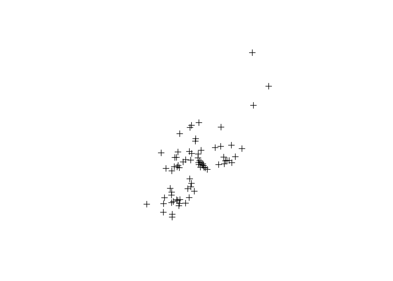
tvpaga.shp <- st_make_valid(tvpaga.shp)
tvpaga.shp <- as_Spatial(tvpaga.shp)

# Plotar o mapa
plot(tvpaga.shp)

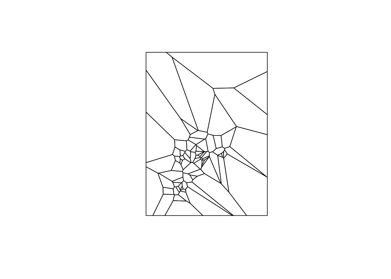
B Importar matriz criada no Geoda

Matrizes criadas no Geoda através de polígonos de Voronoi.

library(spdep)

Loading required package: spData

To access larger datasets in this package, install the spDataLarge
package with: `install.packages('spDataLarge',
repos='https://nowosad.github.io/drat/', type='source')`

queen_nb <- read.gal(file = "data/tvpaga_queen.gal")
queen_w <- nb2listw(neighbours = queen_nb, style = "W")

rook_nb <- read.gal(file = "data/tvpaga_rook.gal")
rook_w <- nb2listw(neighbours = rook_nb, style = "W")

B.1 Teste da importação

summary(queen_nb)

Neighbour list object:
Number of regions: 74 
Number of nonzero links: 404 
Percentage nonzero weights: 7.377648 
Average number of links: 5.459459 
Link number distribution:

 2  3  4  5  6  7  8  9 
 1  3 17 18 18 10  6  1 
1 least connected region:
73 with 2 links
1 most connected region:
33 with 9 links

summary(rook_nb)

Neighbour list object:
Number of regions: 74 
Number of nonzero links: 404 
Percentage nonzero weights: 7.377648 
Average number of links: 5.459459 
Link number distribution:

 2  3  4  5  6  7  8  9 
 1  3 17 18 18 10  6  1 
1 least connected region:
73 with 2 links
1 most connected region:
33 with 9 links

moran.test(x = tvpaga.shp@data$GIN, listw = queen_w)

    Moran I test under randomisation

data:  tvpaga.shp@data$GIN  
weights: queen_w    

Moran I statistic standard deviate = 0.59822, p-value = 0.2748
alternative hypothesis: greater
sample estimates:
Moran I statistic       Expectation          Variance 
    -1.141553e-02     -1.369863e-02      1.456567e-05 

moran.test(x = tvpaga.shp@data$GIN, listw = rook_w)

    Moran I test under randomisation

data:  tvpaga.shp@data$GIN  
weights: rook_w    

Moran I statistic standard deviate = 0.59822, p-value = 0.2748
alternative hypothesis: greater
sample estimates:
Moran I statistic       Expectation          Variance 
    -1.141553e-02     -1.369863e-02      1.456567e-05 

B.2 Criando os polígonos no R

library(dismo)

Loading required package: raster

coordenadas <- coordinates(obj = tvpaga.shp)

tvpaga_voronoi <- voronoi(coordenadas)

plot(tvpaga_voronoi)

B.2.1 Matriz

# Matriz queen
w1 <- nb2listw(poly2nb(tvpaga_voronoi, queen = TRUE), style = "W")

B.2.2 Comparação

moran.test(x = tvpaga.shp@data$GIN, listw = queen_w)

    Moran I test under randomisation

data:  tvpaga.shp@data$GIN  
weights: queen_w    

Moran I statistic standard deviate = 0.59822, p-value = 0.2748
alternative hypothesis: greater
sample estimates:
Moran I statistic       Expectation          Variance 
    -1.141553e-02     -1.369863e-02      1.456567e-05 

moran.test(x = tvpaga.shp@data$GIN, listw = w1)

    Moran I test under randomisation

data:  tvpaga.shp@data$GIN  
weights: w1    

Moran I statistic standard deviate = 0.61642, p-value = 0.2688
alternative hypothesis: greater
sample estimates:
Moran I statistic       Expectation          Variance 
    -1.141553e-02     -1.369863e-02      1.371827e-05