Raw cases

Author

Raphael Saldanha

Last modification

December 1, 2023 | 09:07:18 +01:00

This notebook aims to cluster the Brazilian municipalities considering dengue raw cases time-series similarities.

Packages

library(tidyverse)
library(lubridate)
library(arrow)
library(timetk)
library(dtwclust)
library(kableExtra)
library(tictoc)
source("../functions.R")

Load data

Load the bundled data.

tdengue <- open_dataset(sources = data_dir("bundled_data/tdengue.parquet")) %>%
    select(mun, date, cases = cases_raw) %>%
    collect()

dim(tdengue)

[1] 340179      3

Prepare data

The chunk bellow formats the dataset for tsclust use.

tdengue <- tdengue %>%
  # Prepare time series
  arrange(mun) %>%
  pivot_wider(names_from = mun, values_from = cases) %>%
  select(-date) %>%
  t() %>%
  # Convert object
  tslist()

length(tdengue)

[1] 679

Clustering

Sequence of k groups to be used.

k_seq <- 2:10

DTW (basic)

tic()
clust_dtw <- tsclust(
  series = tdengue, 
  type = "partitional", 
  k = k_seq,
  distance = "dtw_basic",
  seed = 13
)
toc()

46.292 sec elapsed

names(clust_dtw) <- paste0("k_", k_seq)
res_cvi <- sapply(clust_dtw, cvi, type = "internal") %>% 
  t() %>%
  as_tibble(rownames = "k") %>%
  arrange(-Sil)

res_cvi %>%
  gt::gt()

k	Sil	CH	DB	DBstar	D	COP
k_2	0.563306808	243.13362	2.777906	2.777906	4.033050e-03	0.81493978
k_3	0.500486555	179.80850	2.589921	8.236031	3.463657e-03	0.06040454
k_5	0.234604708	102.69761	2.868848	23.661427	7.946198e-04	0.05528690
k_4	0.221410311	122.82411	2.535349	24.240538	7.813649e-04	0.07362652
k_8	0.047380416	71.53960	3.385318	105.686817	3.503914e-04	0.06330307
k_7	0.018931701	66.01800	3.523758	87.921436	2.131907e-04	0.06658659
k_10	-0.005982317	52.35818	3.393992	207.433508	1.469383e-04	0.03558253
k_9	-0.011726942	64.19814	3.436507	244.767080	1.527283e-04	0.02848551
k_6	-0.101115607	73.21168	4.166345	409.352091	1.633515e-05	0.06955750

sel_clust <- clust_dtw[[res_cvi[[1,1]]]]

plot(sel_clust)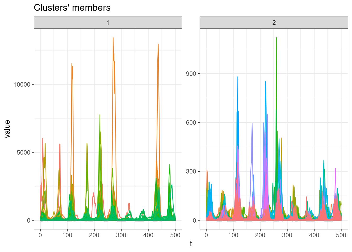

plot(sel_clust, type = "centroids", lty = 1)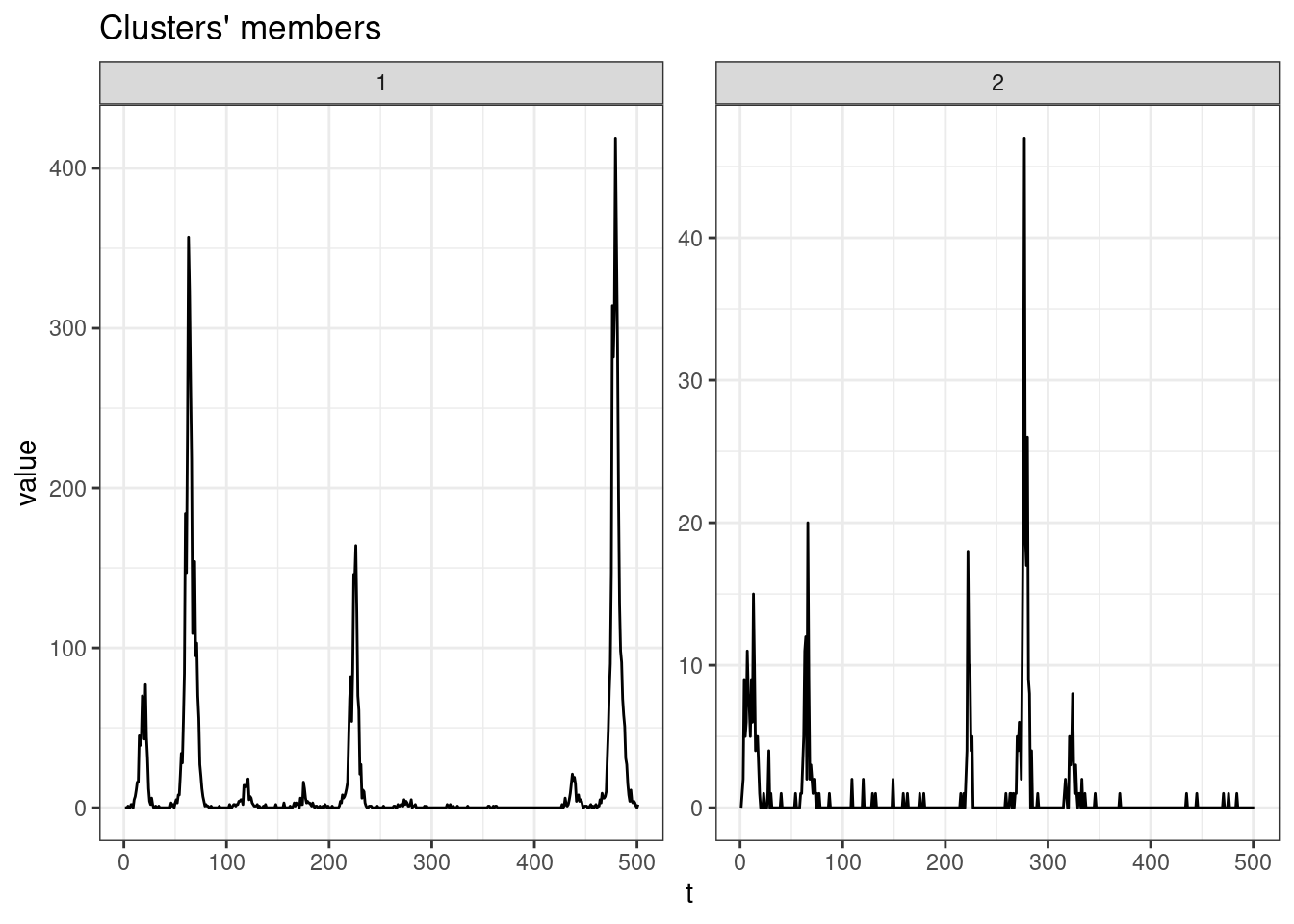

table(sel_clust@cluster)


  1   2 
187 492

Soft-DTW

tic()
clust_sdtw <- tsclust(
  series = tdengue, 
  type = "partitional", 
  k = k_seq,
  distance = "sdtw",
  seed = 13
)
toc()

231.662 sec elapsed

names(clust_sdtw) <- paste0("k_", k_seq)
res_cvi <- sapply(clust_sdtw, cvi, type = "internal") %>% 
  t() %>%
  as_tibble(rownames = "k") %>%
  arrange(-Sil)

res_cvi %>%
  gt::gt()

k	Sil	CH	DB	DBstar	D	COP
k_2	0.9747238	610.6681	0.7127038	7.127038e-01	6.394018e-03	0.021962268
k_3	0.8785473	339.7721	1.3846248	2.184955e+01	6.047589e-05	0.012882348
k_4	0.7831408	367.3748	1.0620911	8.628989e+01	3.151199e-05	0.006517102
k_5	0.5616851	287.9459	1.6410825	6.279292e+02	3.508382e-06	0.006502140
k_6	0.4127518	232.3673	1.8248896	1.900511e+03	1.029877e-06	0.006496556
k_9	0.3492449	161.4531	2.1597151	6.103722e+03	5.179334e-07	0.006423601
k_8	0.3130712	165.0773	2.5475305	5.893653e+03	6.826592e-07	0.006458184
k_7	0.1779085	192.9691	2.0300445	3.657527e+04	1.456487e-07	0.006500423
k_10	0.1726132	130.6724	1.9249465	1.215560e+05	7.778736e-08	0.006444721

sel_clust <- clust_sdtw[[res_cvi[[1,1]]]]

plot(sel_clust)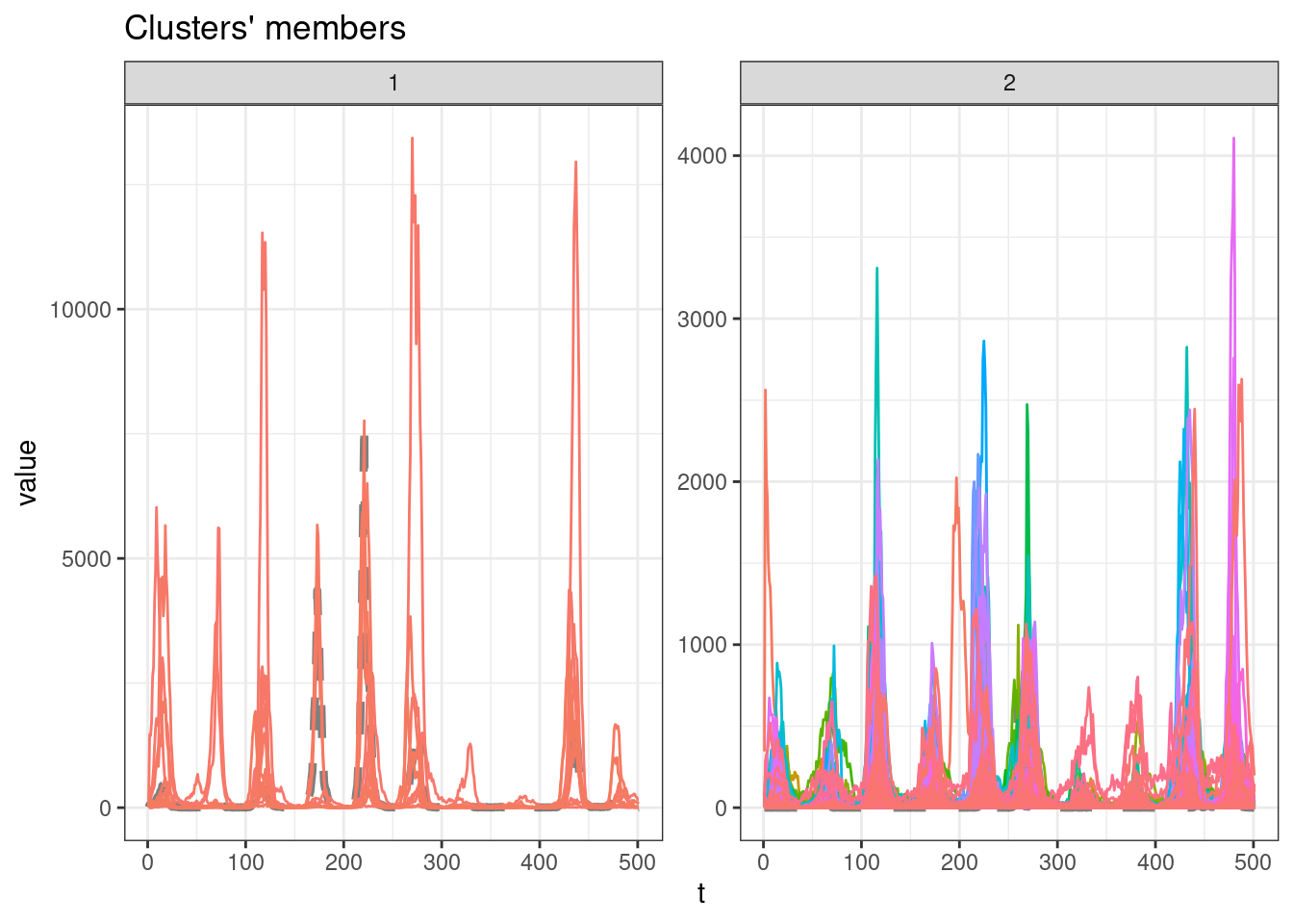

plot(sel_clust, type = "centroids", lty = 1)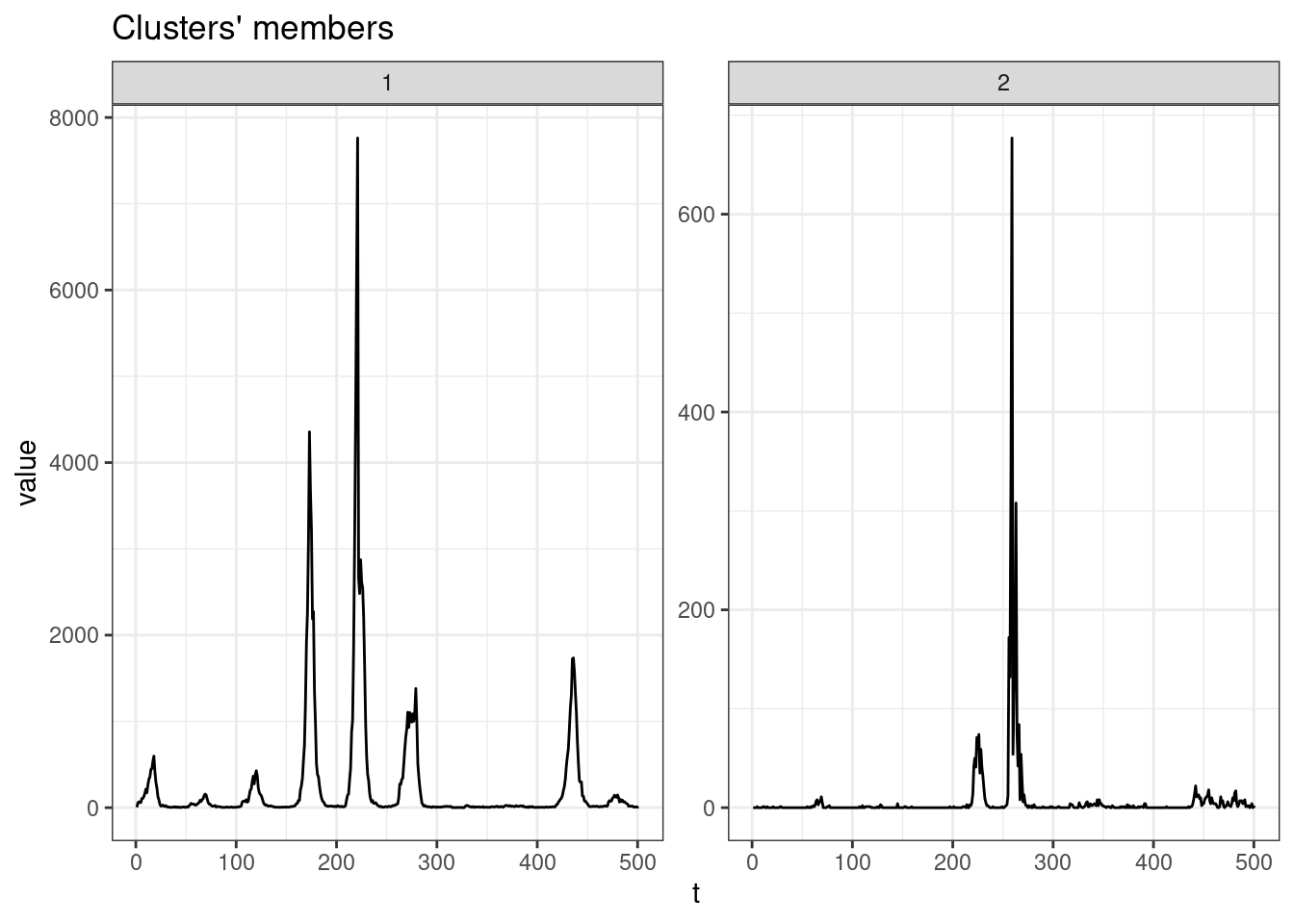

table(sel_clust@cluster)


  1   2 
 11 668

SBD

tic()
clust_sbd <- tsclust(
  series = tdengue, 
  type = "partitional", 
  k = k_seq,
  distance = "sbd",
  seed = 13
)
toc()

0.945 sec elapsed

names(clust_sbd) <- paste0("k_", k_seq)
res_cvi <- sapply(clust_sbd, cvi, type = "internal") %>% 
  t() %>%
  as_tibble(rownames = "k") %>%
  arrange(-Sil)

res_cvi %>%
  gt::gt()

k	Sil	SF	CH	DB	DBstar	D	COP
k_2	0.19232458	0.43352764	105.89969	3.495106	3.495106	0.04758953	0.3749125
k_6	0.16139544	0.14186007	42.69029	3.539215	3.955084	0.05571189	0.3521767
k_5	0.13008017	0.20138965	70.46372	2.731617	3.777455	0.05647432	0.3400697
k_10	0.09211874	0.04440823	49.64036	2.799473	4.241962	0.05073587	0.3159727
k_3	0.08978010	0.31394588	37.06136	6.461761	7.845973	0.02136961	0.3667538
k_9	0.05631414	0.06024602	55.09867	2.170914	3.178624	0.01656789	0.3179895
k_4	0.04322383	0.28795370	96.18451	4.350614	4.857858	0.01715419	0.3501107
k_8	0.03766029	0.08963975	48.19501	3.360877	4.869244	0.01731394	0.3257173
k_7	0.03553741	0.11301210	70.16402	2.846658	4.211674	0.02132175	0.3251809

sel_clust <- clust_sbd[[res_cvi[[1,1]]]]

plot(sel_clust)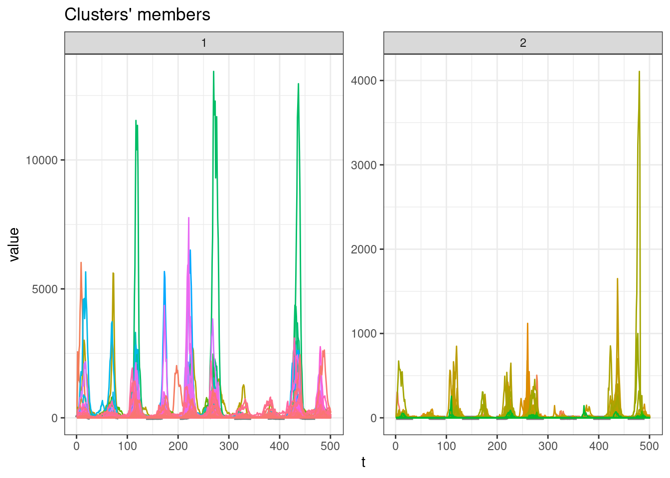

plot(sel_clust, type = "centroids", lty = 1)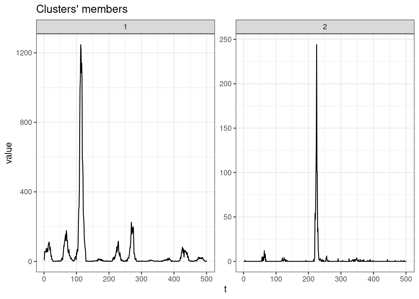

table(sel_clust@cluster)


  1   2 
511 168

GAK

tic()
clust_gak <- tsclust(
  series = tdengue, 
  type = "partitional", 
  k = k_seq,
  distance = "gak",
  seed = 13
)
toc()

271.303 sec elapsed

names(clust_gak) <- paste0("k_", k_seq)
res_cvi <- sapply(clust_gak, cvi, type = "internal") %>% 
  t() %>%
  as_tibble(rownames = "k") %>%
  arrange(-Sil)

res_cvi %>%
  gt::gt()

k	Sil	SF	CH	DB	DBstar	D	COP
k_2	0.91204464	0.6121344	70.160389	11.397435	11.39743	1.070841e-03	0.024308301
k_3	0.89063056	0.6025345	35.827115	12.214961	21.33743	8.882340e-04	0.017392584
k_8	0.56673089	0.5761049	9.540570	36.984617	772.68089	2.073418e-05	0.009652511
k_4	0.51422407	0.6090642	37.881634	9.134131	109.09898	2.369289e-05	0.023596187
k_7	0.34615432	0.5804793	10.401018	24.242925	872.28716	2.770548e-06	0.012348716
k_5	0.32153320	0.5967512	18.167789	15.597700	963.89750	2.566534e-06	0.017167921
k_10	0.30902233	0.5821542	9.743672	20.658947	759.39685	3.587207e-07	0.011523184
k_9	0.19782535	0.5908109	11.123215	20.521645	2053.75182	3.399318e-07	0.019667996
k_6	0.09332721	0.5976834	24.094674	9.259298	1869.00352	3.435826e-07	0.016792580

sel_clust <- clust_gak[[res_cvi[[1,1]]]]

plot(sel_clust)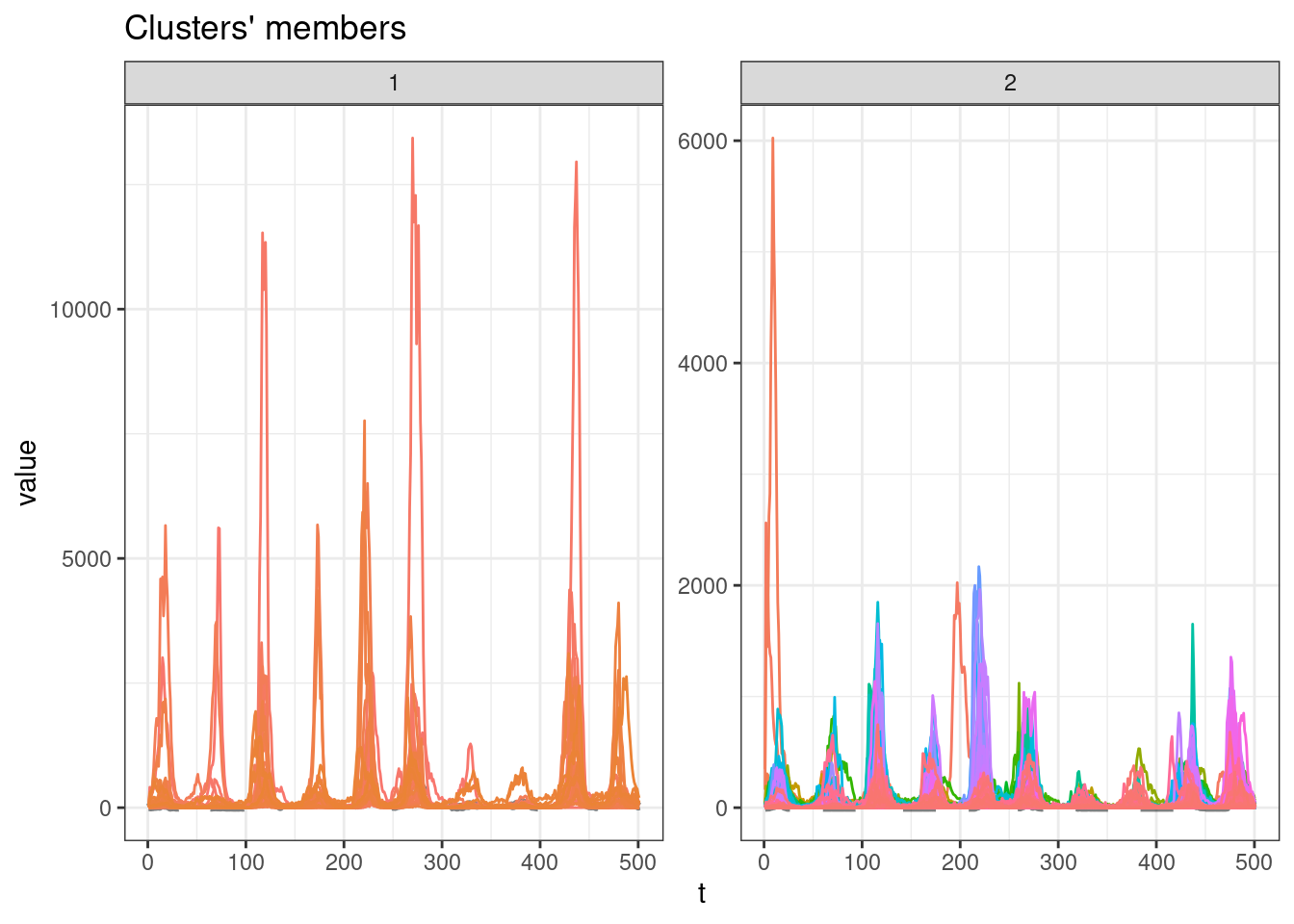

plot(sel_clust, type = "centroids", lty = 1)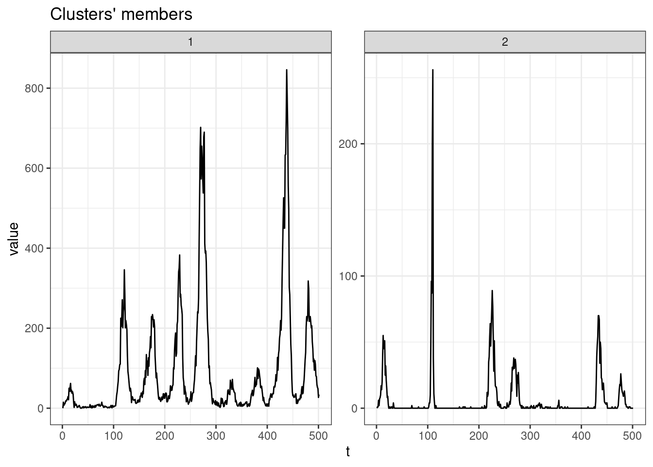

table(sel_clust@cluster)


  1   2 
 32 647

Session info

sessionInfo()

R version 4.3.2 (2023-10-31)
Platform: x86_64-pc-linux-gnu (64-bit)
Running under: Ubuntu 22.04.3 LTS

Matrix products: default
BLAS:   /usr/lib/x86_64-linux-gnu/blas/libblas.so.3.10.0 
LAPACK: /usr/lib/x86_64-linux-gnu/lapack/liblapack.so.3.10.0

Random number generation:
 RNG:     L'Ecuyer-CMRG 
 Normal:  Inversion 
 Sample:  Rejection 
 
locale:
 [1] LC_CTYPE=en_US.UTF-8       LC_NUMERIC=C              
 [3] LC_TIME=en_CA.UTF-8        LC_COLLATE=en_US.UTF-8    
 [5] LC_MONETARY=en_CA.UTF-8    LC_MESSAGES=en_US.UTF-8   
 [7] LC_PAPER=en_CA.UTF-8       LC_NAME=C                 
 [9] LC_ADDRESS=C               LC_TELEPHONE=C            
[11] LC_MEASUREMENT=en_CA.UTF-8 LC_IDENTIFICATION=C       

time zone: Europe/Paris
tzcode source: system (glibc)

attached base packages:
[1] stats     graphics  grDevices utils     datasets  methods   base     

other attached packages:
 [1] tictoc_1.2       kableExtra_1.3.4 dtwclust_5.5.12  dtw_1.23-1      
 [5] proxy_0.4-27     timetk_2.9.0     arrow_13.0.0.1   lubridate_1.9.3 
 [9] forcats_1.0.0    stringr_1.5.0    dplyr_1.1.3      purrr_1.0.2     
[13] readr_2.1.4      tidyr_1.3.0      tibble_3.2.1     ggplot2_3.4.4   
[17] tidyverse_2.0.0 

loaded via a namespace (and not attached):
  [1] rlang_1.1.2         magrittr_2.0.3      clue_0.3-65        
  [4] furrr_0.3.1         flexclust_1.4-1     compiler_4.3.2     
  [7] systemfonts_1.0.5   vctrs_0.6.4         reshape2_1.4.4     
 [10] rvest_1.0.3         lhs_1.1.6           tune_1.1.2         
 [13] pkgconfig_2.0.3     fastmap_1.1.1       ellipsis_0.3.2     
 [16] labeling_0.4.3      utf8_1.2.4          promises_1.2.1     
 [19] rmarkdown_2.25      prodlim_2023.08.28  tzdb_0.4.0         
 [22] bit_4.0.5           xfun_0.41           modeltools_0.2-23  
 [25] jsonlite_1.8.7      recipes_1.0.8       later_1.3.1        
 [28] parallel_4.3.2      cluster_2.1.4       R6_2.5.1           
 [31] stringi_1.7.12      rsample_1.2.0       parallelly_1.36.0  
 [34] rpart_4.1.21        Rcpp_1.0.11         assertthat_0.2.1   
 [37] dials_1.2.0         iterators_1.0.14    knitr_1.45         
 [40] future.apply_1.11.0 zoo_1.8-12          httpuv_1.6.12      
 [43] Matrix_1.6-1.1      splines_4.3.2       nnet_7.3-19        
 [46] timechange_0.2.0    tidyselect_1.2.0    rstudioapi_0.15.0  
 [49] yaml_2.3.7          timeDate_4022.108   codetools_0.2-19   
 [52] listenv_0.9.0       lattice_0.22-5      plyr_1.8.9         
 [55] shiny_1.7.5.1       withr_2.5.2         evaluate_0.23      
 [58] future_1.33.0       survival_3.5-7      RcppParallel_5.1.7 
 [61] xml2_1.3.5          xts_0.13.1          pillar_1.9.0       
 [64] foreach_1.5.2       stats4_4.3.2        shinyjs_2.1.0      
 [67] generics_0.1.3      hms_1.1.3           munsell_0.5.0      
 [70] scales_1.2.1        xtable_1.8-4        globals_0.16.2     
 [73] class_7.3-22        glue_1.6.2          tools_4.3.2        
 [76] data.table_1.14.8   RSpectra_0.16-1     webshot_0.5.5      
 [79] gower_1.0.1         grid_4.3.2          yardstick_1.2.0    
 [82] ipred_0.9-14        colorspace_2.1-0    cli_3.6.1          
 [85] DiceDesign_1.9      workflows_1.1.3     parsnip_1.1.1      
 [88] fansi_1.0.5         viridisLite_0.4.2   gt_0.10.0          
 [91] svglite_2.1.2       lava_1.7.3          gtable_0.3.4       
 [94] GPfit_1.0-8         sass_0.4.7          digest_0.6.33      
 [97] ggrepel_0.9.4       farver_2.1.1        htmlwidgets_1.6.2  
[100] htmltools_0.5.7     lifecycle_1.0.4     httr_1.4.7         
[103] hardhat_1.3.0       mime_0.12           bit64_4.0.5        
[106] MASS_7.3-60