library(tidyverse)
library(arrow)
library(tidymodels)
library(bonsai)
library(finetune)
library(modeltime)
library(timetk)
library(tsfeatures)
library(sparcl)
library(kableExtra)
library(tictoc)
library(geobr)
library(DT)Time series features clustering, with robust sparse k-means
This notebooks aims to implement the global and subset modelling, adopting a clustering strategy based on time series features extraction, with the {tsfeatures} package.
An interesting approach to cluster time series based on feature extraction may be found on Tiano, Bonifati, and Ng (2021). We approximate this strategy by using a robust implementation of sparse \(k\)-means clustering (Witten and Tibshirani 2010; Kondo, Salibian-Barrera, and Zamar 2012).
Packages
Load data
tdengue <- read_parquet(file = "../tdengue.parquet") %>%
  drop_na() %>%
  select(mun, date, starts_with("cases"))
Note
NA values are created when the lagged variables were calculated. The rows containing those NA values are dropped due machine learning regressors constraints.
For validation purposes, only the
casesandcases_lag*covariates variables are keep.
glimpse(tdengue)Rows: 161,370
Columns: 9
$ mun <chr> "110002", "110002", "110002", "110002", "110002", "110002",…
$ date <date> 2011-02-06, 2011-02-13, 2011-02-20, 2011-02-27, 2011-03-06…
$ cases <dbl> -0.51044592, 0.07880156, 0.66804904, 0.07880156, -0.5104459…
$ cases_lag1 <dbl> 2.43579149, -0.51044592, 0.07880156, 0.66804904, 0.07880156…
$ cases_lag2 <dbl> 0.66804904, 2.43579149, -0.51044592, 0.07880156, 0.66804904…
$ cases_lag3 <dbl> 0.07880156, 0.66804904, 2.43579149, -0.51044592, 0.07880156…
$ cases_lag4 <dbl> 0.66804904, 0.07880156, 0.66804904, 2.43579149, -0.51044592…
$ cases_lag5 <dbl> 0.66804904, 0.66804904, 0.07880156, 0.66804904, 2.43579149,…
$ cases_lag6 <dbl> -0.51044592, 0.66804904, 0.66804904, 0.07880156, 0.66804904…Clustering
This procedure goal is to cluster the municipalities considering time series features similarities.
Prepare data
Prepare the data for use with the {tsfeatures} package, converting the panel data to a list of ts objects.
tdengue_df <- tdengue %>%
  arrange(mun, date) %>%
  select(-date) %>%
  nest(data = cases, .by = mun)

tdengue_list <- lapply(tdengue_df$data, ts)
Time series features
Extract time series features.
tsf <- tsfeatures(
  tslist = tdengue_list,
  features = c("entropy", "stability", "lumpiness", "flat_spots", "stl_features", "acf_features")
  )
tsf$mun <- tdengue_df$mun
Robust sparse k-means clustering
Cluster the municipalities based solely on the time series features.
points <- tsf %>%
  select(-mun, -nperiods, -seasonal_period) %>%
  as.matrix() %>%
  scale()
Uses \(k\) from 2 to 10 for clustering.
k_seq <- 2:10cluster_results <- tibble()
cluster_labels <- list()
for(k in k_seq){
res <- RSKC::RSKC(d = points, alpha = 10/60, L1 = NULL, ncl = k)
tmp <- list(list(labels = res$labels))
names(tmp) <- k
cluster_labels <- append(cluster_labels, tmp)
cluster_results <- bind_rows(cluster_results, tibble(k = k, wss = res$WSS))
}The total sum of squares is plotted. The $k=5$ seems to be a break point.
ggplot(cluster_results, aes(k, wss)) +
  geom_line() +
  geom_point() +
  theme_bw()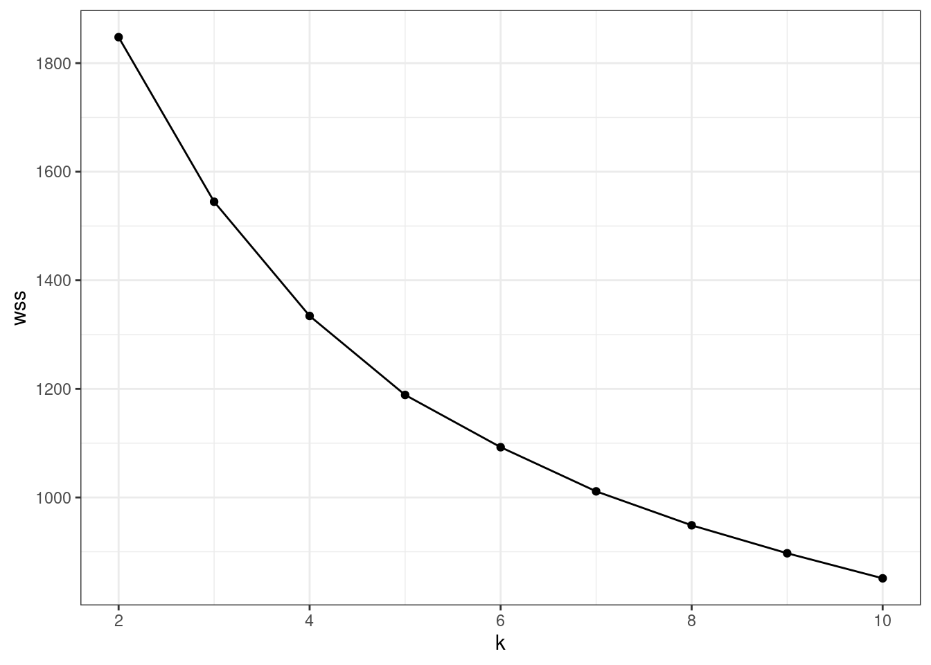
Identify municipalities and cluster id
Finally, the cluster partition ID is added to the main dataset.
cluster_ids <- tibble(
  mun = tdengue_df$mun,
  group = cluster_labels[["5"]]$labels
)
tdengue <- left_join(tdengue, cluster_ids, by = "mun")Cluster sizes
table(cluster_ids$group)
 1  2  3  4  5
38 92 80 84 32
Train and test split
Split the data into training and testing. The function time_series_split handles the time series, not shuffling them, and considering the panel data format, as depicted in the message about overlapping timestamps detected.
The last two years data will be used as the training set.
tdengue_split <- tdengue %>%
  time_series_split(
    date_var = date,
    assess = 52*2,
    cumulative = TRUE
  )
Data is not ordered by the 'date_var'. Resamples will be arranged by `date`.Overlapping Timestamps Detected. Processing overlapping time series together using sliding windows.tdengue_split<Analysis/Assess/Total>
<127466/33904/161370>K-folds
The training set will be split into k folds.
tdengue_split_folds <- training(tdengue_split) %>%
  vfold_cv(v = 5)
Recipes
The global and subset models training specification are called recipes. The procedure bellow creates a list of those recipes.
recipes_list <- list()Global
The global training recipe uses data from all municipalities for training the models.
The date and group variables are removed prior training
The municipality identification variable is treated as an Id variable, taking no place as a predictor in the training process
recipe_global <- recipe(cases ~ ., data = training(tdengue_split)) %>%
  step_rm(date, group) %>%
  update_role(mun, new_role = "id variable")

recipes_list <- append(recipes_list, list(global = recipe_global))

rm(recipe_global)
Groups
For each group created by the clustering process, a specific training recipe will be created. For this, the first step is to filter rows from the training set, keep only the rows belonging to the group in the loop
The date and group variables are removed prior training
The municipality identification variable is treated as an Id variable, taking no place as a predictor in the training process
for(g in unique(tdengue$group)){
  tmp <- recipe(cases ~ ., data = training(tdengue_split)) %>%
    step_filter(group == !!g) %>%
    step_rm(date, group) %>%
    update_role(mun, new_role = "id variable")

  tmp <- list(tmp)
  tmp <- setNames(tmp, paste0("g", g))

  recipes_list <- append(recipes_list, tmp)

  rm(tmp)
}
Regressors specification
Random forest
A Random Forest specification using the ranger engine. The trees and min_n hyperparameters will be tuned.
rf_spec <- rand_forest(
  trees = tune(),
  min_n = tune()
) %>%
  set_engine("ranger") %>%
  set_mode("regression")
LightGBM
# lgbm_spec <- boost_tree(
#   trees = tune(),
#   min_n = tune(),
#   tree_depth = tune()
# ) %>%
#   set_engine("lightgbm") %>%
#   set_mode("regression")
Workflow set
This step creates a workflow set, combining the training recipes and regressors specifications.
all_workflows <- workflow_set(
  preproc = recipes_list,
  models = list(rf = rf_spec),
  cross = TRUE
)
Tune
This step tunes the training hyperparameters of each workflow.
doParallel::registerDoParallel()

tic()
race_results <-
  all_workflows %>%
  workflow_map(
    "tune_race_anova",
    seed = 345,
    resamples = tdengue_split_folds,
    grid = 10,
    control = control_race(parallel_over = "everything"),
    verbose = TRUE
  )
i 1 of 6 tuning: global_rf✔ 1 of 6 tuning: global_rf (29m 42.5s)i 2 of 6 tuning: g3_rf✔ 2 of 6 tuning: g3_rf (3m 8.8s)i 3 of 6 tuning: g1_rf✔ 3 of 6 tuning: g1_rf (1m 39s)i 4 of 6 tuning: g4_rf✔ 4 of 6 tuning: g4_rf (4m 14.5s)i 5 of 6 tuning: g2_rf✔ 5 of 6 tuning: g2_rf (5m 57.4s)i 6 of 6 tuning: g5_rf✔ 6 of 6 tuning: g5_rf (37.6s)toc()2721.037 sec elapsedFit
Each workflow will be trained using the tuned hyperparameters, considering the RMSE metric as reference.
This procedure creates a list of trained models, containing the fit results and a list of the municipalities used on the training of each workflow.
The global workflow is trained with data from all municipalities and the subsets workflows are trained using the respective municipalities list given by the cluster algorithm.
tic()
trained_models <- list()
for(w in unique(race_results$wflow_id)){
  best_tune <- race_results %>%
    extract_workflow_set_result(w) %>%
    select_best("rmse")

  final_fit <- race_results %>%
    extract_workflow(w) %>%
    finalize_workflow(best_tune) %>%
    fit(training(tdengue_split))

  mold <- extract_mold(final_fit)
  train_ids <- mold$extras$roles$`id variable` %>%
    distinct() %>%
    pull() %>%
    as.character()

  final_fit <- list(
    list(
      "final_fit" = final_fit,
      "train_ids" = train_ids
    )
  )

  final_fit <- setNames(final_fit, paste0(w))

  trained_models <- append(trained_models, final_fit)
}
toc()
410.867 sec elapsedAccuracy
After training each workflow, the accuracy of the models are obtained applying the fitted models on the testing set.
For the global model, all municipalities are using for testing. For the subsets models, only data from the subset’s municipalities are considered for testing.
The RMSE metric is obtained for each workflow and municipality.
models_accuracy <- tibble()
for(t in 1:length(trained_models)){

  model_tbl <- modeltime_table(trained_models[[t]][[1]])
  testing_set <- testing(tdengue_split) %>%
    filter(mun %in% trained_models[[t]][[2]])


  calib_tbl <- model_tbl %>%
      modeltime_calibrate(
        new_data = testing_set,
        id       = "mun"
      )

  res <- calib_tbl %>%
      modeltime_accuracy(
        acc_by_id = TRUE,
        metric_set = metric_set(rmse)
      )

  res$.model_id <- word(names(trained_models[t]), 1, sep = "_")

  models_accuracy <- bind_rows(models_accuracy, res)
}
This plot presents the RMSE distribution across the workflows.
ggplot(data = models_accuracy, aes(x = .model_id, y = rmse, fill = .model_desc)) +
  geom_boxplot()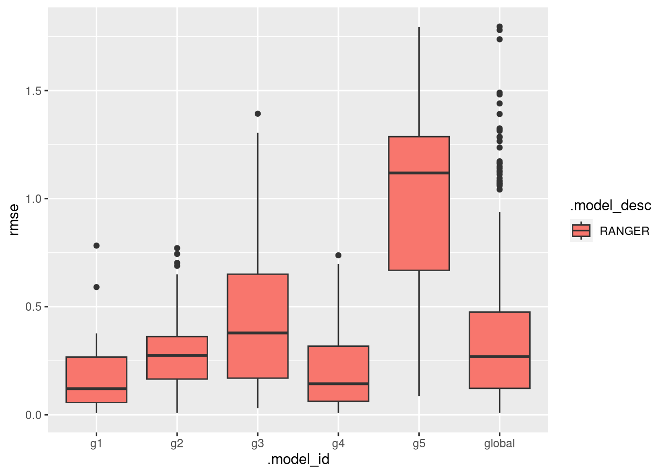
Breakdown
mun_names <- lookup_muni(code_muni = "all") %>%
  mutate(code_muni = substr(code_muni, 0, 6)) %>%
  mutate(name_muni = paste0(name_muni, ", ", abbrev_state)) %>%
  select(code_muni, name_muni)
Using year 2010models_accuracy %>%
left_join(mun_names, by = c("mun" = "code_muni")) %>%
select(.model_id, .model_desc, name_muni, rmse) %>%
mutate(rmse = round(rmse, 2)) %>%
arrange(.model_id, .model_desc, -rmse) %>%
datatable(filter = "top")models_accuracy %>%
left_join(mun_names, by = c("mun" = "code_muni")) %>%
select(.model_id, .model_desc, name_muni, rmse) %>%
mutate(rmse = round(rmse, 2)) %>%
group_by(.model_desc) %>%
mutate(.model_id = case_when(
.model_id != "global" ~ "cluster",
.default = .model_id
)) %>%
pivot_wider(names_from = .model_id, values_from = rmse) %>%
mutate(dif = round(global - cluster, 2)) %>%
ungroup() %>%
datatable(filter = "top")Session info
sessionInfo()R version 4.1.2 (2021-11-01)
Platform: x86_64-pc-linux-gnu (64-bit)
Running under: Ubuntu 22.04.2 LTS
Matrix products: default
BLAS: /usr/lib/x86_64-linux-gnu/blas/libblas.so.3.10.0
LAPACK: /usr/lib/x86_64-linux-gnu/lapack/liblapack.so.3.10.0
locale:
[1] LC_CTYPE=pt_BR.UTF-8 LC_NUMERIC=C
[3] LC_TIME=en_US.UTF-8 LC_COLLATE=en_US.UTF-8
[5] LC_MONETARY=en_US.UTF-8 LC_MESSAGES=en_US.UTF-8
[7] LC_PAPER=en_US.UTF-8 LC_NAME=C
[9] LC_ADDRESS=C LC_TELEPHONE=C
[11] LC_MEASUREMENT=en_US.UTF-8 LC_IDENTIFICATION=C
attached base packages:
[1] stats graphics grDevices utils datasets methods base
other attached packages:
[1] rlang_1.1.1 ranger_0.15.1 DT_0.28 geobr_1.7.0
[5] tictoc_1.2 kableExtra_1.3.4 sparcl_1.0.4 tsfeatures_1.1
[9] timetk_2.8.3 modeltime_1.2.7 finetune_1.1.0 bonsai_0.2.1
[13] yardstick_1.2.0 workflowsets_1.0.1 workflows_1.1.3 tune_1.1.1
[17] rsample_1.1.1 recipes_1.0.6 parsnip_1.1.0 modeldata_1.1.0
[21] infer_1.0.4 dials_1.2.0 scales_1.2.1 broom_1.0.5
[25] tidymodels_1.1.0 arrow_12.0.1 lubridate_1.9.2 forcats_1.0.0
[29] stringr_1.5.0 dplyr_1.1.2 purrr_1.0.1 readr_2.1.4
[33] tidyr_1.3.0 tibble_3.2.1 ggplot2_3.4.2 tidyverse_2.0.0
loaded via a namespace (and not attached):
[1] backports_1.4.1 systemfonts_1.0.4 splines_4.1.2
[4] crosstalk_1.2.0 listenv_0.9.0 digest_0.6.33
[7] foreach_1.5.2 htmltools_0.5.5 fansi_1.0.4
[10] magrittr_2.0.3 doParallel_1.0.17 tzdb_0.4.0
[13] globals_0.16.2 gower_1.0.1 RcppParallel_5.1.7
[16] xts_0.13.1 svglite_2.1.1 hardhat_1.3.0
[19] timechange_0.2.0 prettyunits_1.1.1 forecast_8.21
[22] tseries_0.10-54 colorspace_2.1-0 rvest_1.0.3
[25] xfun_0.39 jsonlite_1.8.7 lme4_1.1-34
[28] survival_3.2-13 zoo_1.8-12 iterators_1.0.14
[31] glue_1.6.2 gtable_0.3.3 ipred_0.9-14
[34] webshot_0.5.5 RSKC_2.4.2 future.apply_1.11.0
[37] quantmod_0.4.23 DBI_1.1.3 Rcpp_1.0.11
[40] viridisLite_0.4.2 units_0.8-2 GPfit_1.0-8
[43] bit_4.0.5 proxy_0.4-27 stats4_4.1.2
[46] lava_1.7.2.1 StanHeaders_2.26.27 prodlim_2023.03.31
[49] htmlwidgets_1.6.2 httr_1.4.6 ellipsis_0.3.2
[52] modeltools_0.2-23 farver_2.1.1 pkgconfig_2.0.3
[55] sass_0.4.6 nnet_7.3-17 utf8_1.2.3
[58] labeling_0.4.2 tidyselect_1.2.0 DiceDesign_1.9
[61] cachem_1.0.8 munsell_0.5.0 tools_4.1.2
[64] cli_3.6.1 generics_0.1.3 evaluate_0.21
[67] fastmap_1.1.1 yaml_2.3.7 knitr_1.43
[70] bit64_4.0.5 future_1.33.0 nlme_3.1-155
[73] xml2_1.3.5 flexclust_1.4-1 compiler_4.1.2
[76] rstudioapi_0.15.0 curl_5.0.1 e1071_1.7-13
[79] lhs_1.1.6 bslib_0.5.0 stringi_1.7.12
[82] lattice_0.20-45 Matrix_1.6-0 nloptr_2.0.3
[85] classInt_0.4-9 urca_1.3-3 vctrs_0.6.3
[88] pillar_1.9.0 lifecycle_1.0.3 furrr_0.3.1
[91] jquerylib_0.1.4 lmtest_0.9-40 data.table_1.14.8
[94] R6_2.5.1 KernSmooth_2.23-20 parallelly_1.36.0
[97] codetools_0.2-18 boot_1.3-28 MASS_7.3-55
[100] assertthat_0.2.1 withr_2.5.0 fracdiff_1.5-2
[103] parallel_4.1.2 hms_1.1.3 quadprog_1.5-8
[106] grid_4.1.2 rpart_4.1.16 timeDate_4022.108
[109] minqa_1.2.5 class_7.3-20 rmarkdown_2.23
[112] TTR_0.24.3 sf_1.0-13 Links of intererest
References
Kondo, Yumi, Matias Salibian-Barrera, and Ruben Zamar. 2012. “A Robust and Sparse K-Means Clustering Algorithm,” January. http://arxiv.org/abs/1201.6082.
Tiano, Donato, Angela Bonifati, and Raymond Ng. 2021. “Feature-Driven Time Series Clustering.” https://doi.org/10.5441/002/EDBT.2021.33.
Witten, Daniela M., and Robert Tibshirani. 2010. “A Framework for Feature Selection in Clustering.” Journal of the American Statistical Association 105 (490): 713–26. https://doi.org/10.1198/jasa.2010.tm09415.