Denque and weather lags

Author

Raphael Saldanha

Last modification

January 25, 2024 | 15:18:06 +01:00

This notebook aims to study the relationship between Dengue cases incidence with lagged climate indicators, specially the co-occurrence of specific climate conditions that precedes an outbreak.

Packages

library(tidyverse)
library(tidymodels)
library(hotspots)
library(DT)
library(finetune)
library(themis)
library(arrow)
library(timetk)
library(rpart.plot)
library(vip)
library(doParallel)
doParallel::registerDoParallel()

source("../functions.R")

Dataset construction

Dengue

code_muni <- 3136702 # Juiz de Fora, MG

The original data on municipality dengue cases incidence present daily observations and is summarized by month.

dengue_df <- open_dataset(data_dir("dengue_data/parquet_aggregated/dengue_md.parquet")) %>%
  filter(mun == !!substr(code_muni, 0, 6)) %>%
  collect() %>%
  summarise_by_time(.date_var = date, .by = "month", freq = sum(freq, na.rm = TRUE))

Classify

Based on the observed frequency distribution of cases, we classify the months as anomalous or not.

hot_ref <- hotspots(
  x = dengue_df$freq, 
  p = 0.99, 
  var.est = "mad",
)$positive.cut

dengue_df_anom <- dengue_df %>%
  mutate(anomaly = if_else(freq >= hot_ref, TRUE, FALSE)) %>%
  mutate(anomaly = as.factor(anomaly))

dengue_df_anom %>%
  ggplot(aes(x = date, y = freq, fill = anomaly)) +
  geom_bar(stat = "identity") +
  scale_fill_discrete(direction = -1) +
  theme(
    legend.position = "bottom",
    legend.direction = "horizontal"
  )

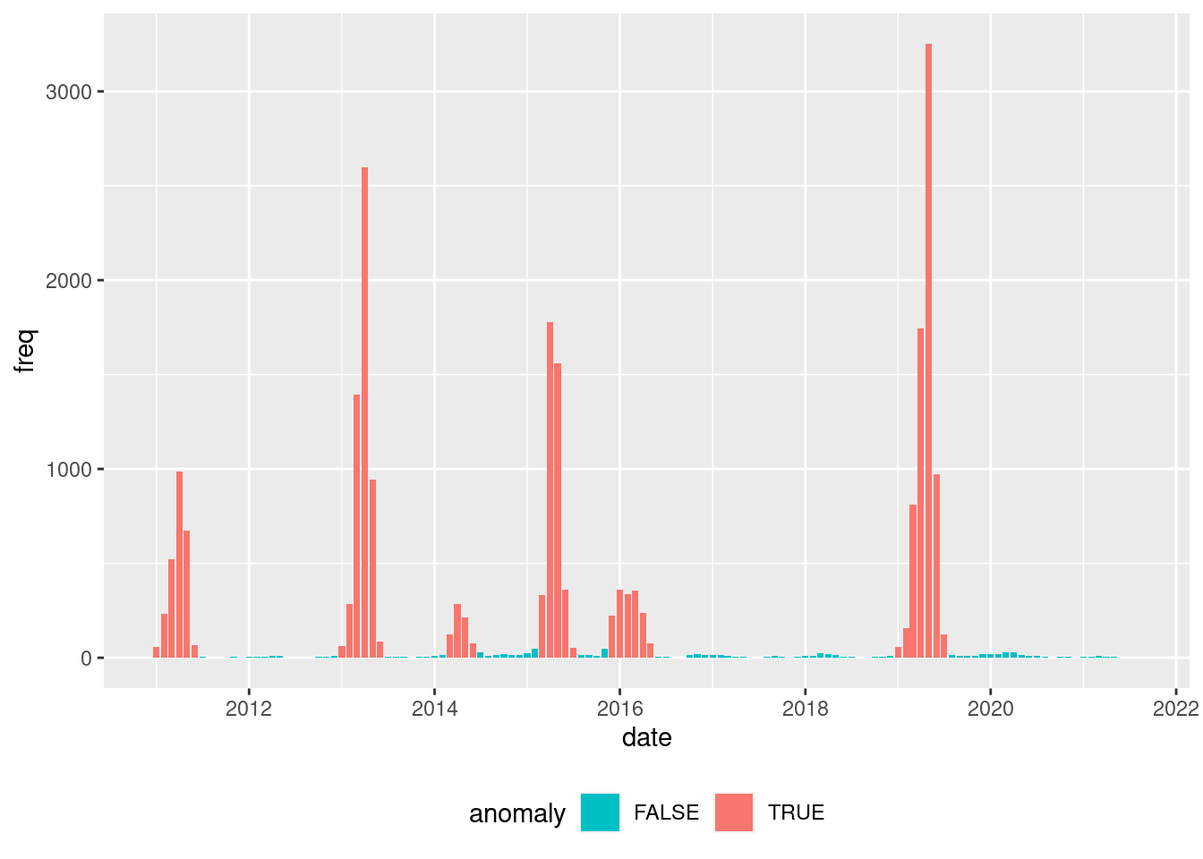
dengue_df <- inner_join(dengue_df, dengue_df_anom)

Joining with `by = join_by(date, freq)`

Proportion table of anomalous (yes) and not anomalous (not) months.

prop.table(table(dengue_df$anomaly))


   FALSE     TRUE 
0.734375 0.265625

Weather data

The available weather data is also originally presented in daily observations and aggregate to months. For temperature indicators, the mean is used, for precipitation, the sum is used for aggregation.

tmax <- open_dataset(sources = data_dir("weather_data/parquet/brdwgd/tmax.parquet")) %>%
  filter(code_muni == code_muni) %>%
  filter(name == "Tmax_mean") %>%
  select(date, value) %>%
  collect() %>%
  filter(date >= min(dengue_df$date) & date <= max(dengue_df$date)) %>%
  summarise_by_time(.date_var = date, .by = "month", value = mean(value, na.rm = TRUE)) %>%
  rename(tmax = value)

tmin <- open_dataset(sources = data_dir("weather_data/parquet/brdwgd/tmin.parquet")) %>%
  filter(code_muni == code_muni) %>%
  filter(name == "Tmin_mean") %>%
  select(date, value) %>%
  collect() %>%
  filter(date >= min(dengue_df$date) & date <= max(dengue_df$date)) %>%
  summarise_by_time(.date_var = date, .by = "month", value = mean(value, na.rm = TRUE)) %>%
  rename(tmin = value)

prec <- open_dataset(sources = data_dir("weather_data/parquet/brdwgd/pr.parquet")) %>%
  filter(code_muni == code_muni) %>%
  filter(name == "pr_sum") %>%
  select(date, value) %>%
  collect() %>%
  filter(date >= min(dengue_df$date) & date <= max(dengue_df$date)) %>%
  summarise_by_time(.date_var = date, .by = "month", value = sum(value, na.rm = TRUE)) %>%
  rename(prec = value)

Join data

Join dengue and weather datasets.

res <- inner_join(x = dengue_df, y = tmax, by = "date") %>%
  inner_join(tmin, by = "date") %>%
  inner_join(prec, by = "date") %>%
  select(date, anomaly, tmax, tmin, prec)

Time lag

This step produces time lagged variables (from 1 to 6 months) from the weather indicators, remove the date variable, and omit records with missing data (only present after the time lag procedure).

res_prep <- res %>%
  select(-date) %>%
  tk_augment_lags(
    .value = c(tmax, tmin, prec), 
    .lags = 1:6
  ) %>% 
  select(-tmax, -tmin, -prec) %>%
  na.omit()

head(res_prep) %>% datatable()

Dataset split

Splits the dataset into training and testing.

res_split <- initial_time_split(
  data = res_prep, 
  prop = .8, 
  lag = 6
)

train_data <- training(res_split)
test_data <- testing(res_split)

Remove old objects and triggers a memory garbage collection.

rm(dengue_df, dengue_df_anom, res, res_prep)
gc()

          used (Mb) gc trigger   (Mb)  max used   (Mb)
Ncells 3013526  161    4749918  253.7   4749918  253.7
Vcells 5234027   40  403999596 3082.3 679072422 5181.0

Modeling

Recipes

Creates model recipes with the model specitication, data (train dataset). Several recipes are created with different methods to balance the training dataset.

rec_upsample <- 
  recipe(anomaly ~ ., train_data) %>%
  step_upsample(
    anomaly, 
    over_ratio = tune()
  )

rec_rose <- 
  recipe(anomaly ~ ., train_data) %>%
  step_rose(
    anomaly, 
    over_ratio = tune()
  )

rec_smote <- 
  recipe(anomaly ~ ., train_data) %>%
  step_smote(
    anomaly, 
    over_ratio = tune(),
    neighbors = tune()
  )

rec_adasyn <- 
  recipe(anomaly ~ ., train_data) %>%
  step_adasyn(
    anomaly, 
    over_ratio = tune(),
    neighbors = tune()
  )

rec_downsample <- 
  recipe(anomaly ~ ., train_data) %>%
  step_downsample(
    anomaly, 
    under_ratio = tune()
  )

Learners

Decision trees are choose due its directly interpretability and rules extraction. Two learners are created with different engines (rpart and partykit).

tree_rp_spec <- decision_tree(
  cost_complexity = tune(),
  tree_depth = tune(),
  min_n = tune()
) %>%
  set_engine("rpart") %>%
  set_mode("classification")

Folding

Creates a v-fold for cross-validation.

folds <- vfold_cv(
  data = train_data, 
  v = 10, 
  strata = anomaly
)

Workflow setting

This step creates an modeling workflow by combining the recipes and learners options.

wf_set <- 
  workflow_set(
    preproc = list(
      upsample = rec_upsample,
      rose = rec_rose, 
      smote = rec_smote, 
      adasyn = rec_adasyn,
      downsample = rec_downsample
    ),
    models = list(
      dt = tree_rp_spec
    ),
    cross = TRUE
  )

Tuning

This step tune hyper-parameters from the models (learners and balancing steps) using an ANOVA race.

tune_results <- wf_set %>%
  workflow_map(
    "tune_race_anova",
    seed = 345,
    resamples = folds,
    grid = 50,
    metrics = metric_set(
      accuracy, 
      bal_accuracy,
      roc_auc, 
      ppv,
      sens,
      spec
    ),
    control = control_race(parallel_over = "everything"),
    verbose = TRUE
  )

i 1 of 5 tuning:     upsample_dt

✔ 1 of 5 tuning:     upsample_dt (9.4s)

i 2 of 5 tuning:     rose_dt

✔ 2 of 5 tuning:     rose_dt (7.4s)

i 3 of 5 tuning:     smote_dt

✔ 3 of 5 tuning:     smote_dt (9.7s)

i 4 of 5 tuning:     adasyn_dt

✔ 4 of 5 tuning:     adasyn_dt (8s)

i 5 of 5 tuning:     downsample_dt

✔ 5 of 5 tuning:     downsample_dt (10.4s)

Best workflow and model selection

Based on the tuning results, this step identifies the best learner strategy and best model hyper-parameters based on the ROC-AUC metric.

target_metric <- "bal_accuracy"

best_wf <- tune_results %>% 
  rank_results(rank_metric = target_metric) %>% 
  filter(.metric == target_metric) %>% 
  select(wflow_id, model, .config, accuracy = mean, rank) %>%
  slice(1) %>%
  pull(wflow_id)

print(best_wf)

[1] "upsample_dt"

best_tune <- tune_results %>%
  extract_workflow_set_result(id = best_wf) %>%
  select_best(metric = target_metric)

t(best_tune)

                [,1]                   
cost_complexity "0.02850468"           
tree_depth      "9"                    
min_n           "8"                    
over_ratio      "0.8693291"            
.config         "Preprocessor37_Model1"

Finalize workflow

Finalizes the workflow with the choose learner and hyper-parameter combination, performing the last fit of the model with the entire dataset.

fitted_wf <- tune_results %>%
  extract_workflow(id = best_wf) %>%
  finalize_workflow(best_tune) %>%
  last_fit(split = res_split)

Results

Decision tree plot

extracted_engine <-  fitted_wf %>% extract_fit_engine()

rpart.plot(extracted_engine, roundint = FALSE)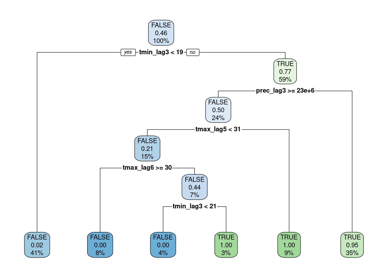

Confusion matrix

augment(fitted_wf) %>%
  conf_mat(truth = anomaly, estimate = .pred_class)

          Truth
Prediction FALSE TRUE
     FALSE    16    1
     TRUE      5    6

Model performance metrics

multi_metric <- metric_set(
  accuracy, 
  bal_accuracy,
  roc_auc, 
  ppv,
  sens,
  spec
)

augment(fitted_wf) %>%
  multi_metric(truth = anomaly, estimate = .pred_class, .pred_TRUE)

# A tibble: 6 × 3
  .metric      .estimator .estimate
  <chr>        <chr>          <dbl>
1 accuracy     binary         0.786
2 bal_accuracy binary         0.810
3 ppv          binary         0.941
4 sens         binary         0.762
5 spec         binary         0.857
6 roc_auc      binary         0.238

Variable importance plot

fitted_wf %>% 
  extract_fit_engine() %>% 
  vip()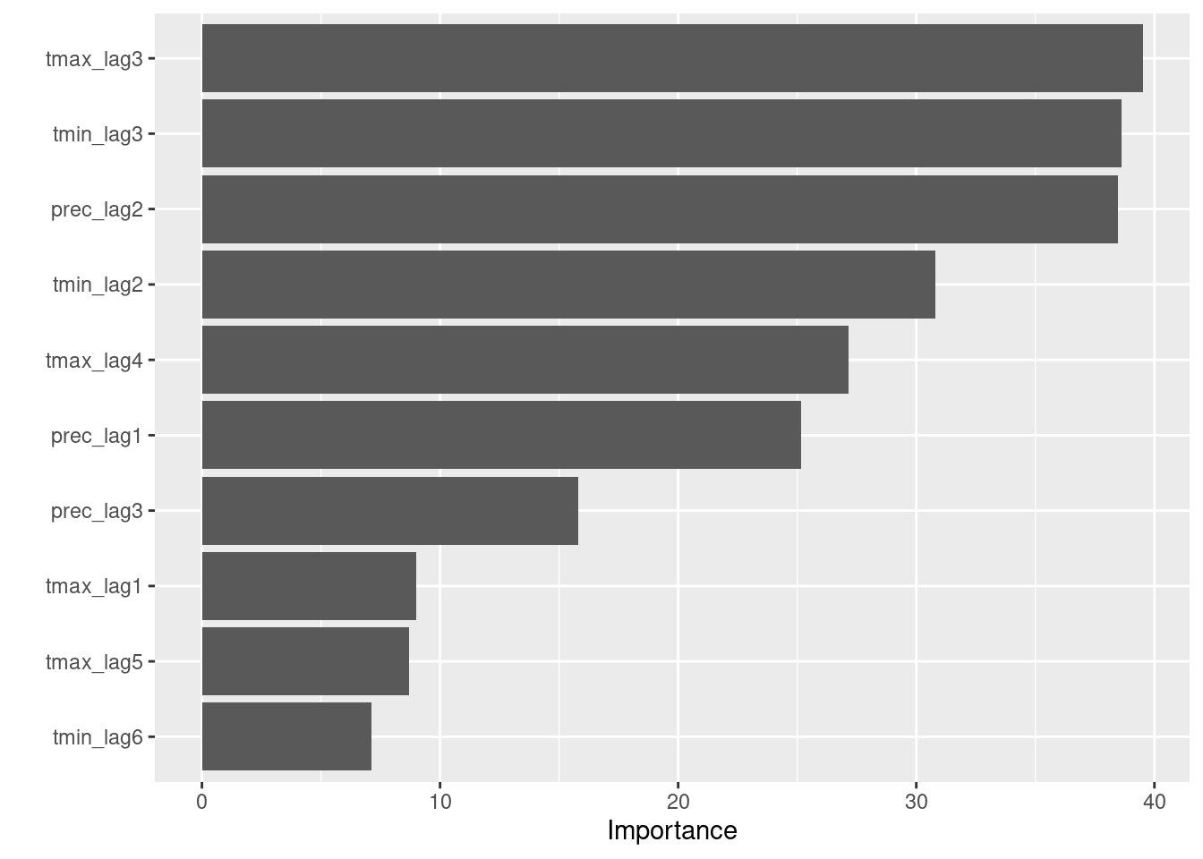

Session info

sessionInfo()

R version 4.3.2 (2023-10-31)
Platform: x86_64-pc-linux-gnu (64-bit)
Running under: Ubuntu 22.04.3 LTS

Matrix products: default
BLAS:   /usr/lib/x86_64-linux-gnu/blas/libblas.so.3.10.0 
LAPACK: /usr/lib/x86_64-linux-gnu/lapack/liblapack.so.3.10.0

locale:
 [1] LC_CTYPE=en_US.UTF-8       LC_NUMERIC=C              
 [3] LC_TIME=en_CA.UTF-8        LC_COLLATE=en_US.UTF-8    
 [5] LC_MONETARY=en_CA.UTF-8    LC_MESSAGES=en_US.UTF-8   
 [7] LC_PAPER=en_CA.UTF-8       LC_NAME=C                 
 [9] LC_ADDRESS=C               LC_TELEPHONE=C            
[11] LC_MEASUREMENT=en_CA.UTF-8 LC_IDENTIFICATION=C       

time zone: Europe/Paris
tzcode source: system (glibc)

attached base packages:
[1] parallel  stats     graphics  grDevices utils     datasets  methods  
[8] base     

other attached packages:
 [1] ROSE_0.0-4         rlang_1.1.3        doParallel_1.0.17  iterators_1.0.14  
 [5] foreach_1.5.2      vip_0.4.1          rpart.plot_3.1.1   rpart_4.1.23      
 [9] timetk_2.9.0       arrow_14.0.0.2     themis_1.0.2       finetune_1.1.0    
[13] DT_0.31            hotspots_1.0.3     ineq_0.2-13        lattice_0.22-5    
[17] yardstick_1.3.0    workflowsets_1.0.1 workflows_1.1.3    tune_1.1.2        
[21] rsample_1.2.0      recipes_1.0.9      parsnip_1.1.1      modeldata_1.3.0   
[25] infer_1.0.5        dials_1.2.0        scales_1.3.0       broom_1.0.5       
[29] tidymodels_1.1.1   lubridate_1.9.3    forcats_1.0.0      stringr_1.5.1     
[33] dplyr_1.1.4        purrr_1.0.2        readr_2.1.5        tidyr_1.3.1       
[37] tibble_3.2.1       ggplot2_3.4.4      tidyverse_2.0.0   

loaded via a namespace (and not attached):
 [1] magrittr_2.0.3      furrr_0.3.1         compiler_4.3.2     
 [4] vctrs_0.6.5         lhs_1.1.6           pkgconfig_2.0.3    
 [7] fastmap_1.1.1       ellipsis_0.3.2      backports_1.4.1    
[10] labeling_0.4.3      utf8_1.2.4          rmarkdown_2.25     
[13] prodlim_2023.08.28  tzdb_0.4.0          nloptr_2.0.3       
[16] bit_4.0.5           xfun_0.41           cachem_1.0.8       
[19] jsonlite_1.8.8      prettyunits_1.2.0   R6_2.5.1           
[22] bslib_0.6.1         stringi_1.8.3       boot_1.3-28        
[25] parallelly_1.36.0   jquerylib_0.1.4     Rcpp_1.0.12        
[28] assertthat_0.2.1    knitr_1.45          future.apply_1.11.1
[31] zoo_1.8-12          Matrix_1.6-3        splines_4.3.2      
[34] nnet_7.3-19         timechange_0.3.0    tidyselect_1.2.0   
[37] rstudioapi_0.15.0   yaml_2.3.8          timeDate_4032.109  
[40] codetools_0.2-19    listenv_0.9.0       withr_3.0.0        
[43] evaluate_0.23       future_1.33.1       survival_3.5-7     
[46] xts_0.13.2          pillar_1.9.0        generics_0.1.3     
[49] hms_1.1.3           munsell_0.5.0       minqa_1.2.6        
[52] globals_0.16.2      class_7.3-22        glue_1.7.0         
[55] tools_4.3.2         data.table_1.14.10  lme4_1.1-35.1      
[58] gower_1.0.1         grid_4.3.2          crosstalk_1.2.1    
[61] ipred_0.9-14        colorspace_2.1-0    nlme_3.1-163       
[64] cli_3.6.2           DiceDesign_1.10     fansi_1.0.6        
[67] lava_1.7.3          gtable_0.3.4        GPfit_1.0-8        
[70] sass_0.4.8          digest_0.6.34       farver_2.1.1       
[73] htmlwidgets_1.6.4   htmltools_0.5.7     lifecycle_1.0.4    
[76] hardhat_1.3.0       bit64_4.0.5         MASS_7.3-60