library(tidyverse)
library(arrow)
library(tidymodels)
library(bonsai)
library(finetune)
library(modeltime)
library(timetk)
library(dtwclust)
library(kableExtra)
library(tictoc)
library(geobr)
library(DT)
library(sf)
source("../functions.R")Multivariate clustering, all data model
This notebooks aims to reproduce the methodology of the paper submitted to the SBD2023 conference, implementing the global and subset modelling with a multivariate approach.
This methodology aims to compare the performance of models trained with data from all municipalities time-series (global models) and models trained with subset of municipalities time-series (subset models).
Those subsets were created by a clustering algorithm considering the cases and climate time-series.
Packages
Load data
tdengue <- read_parquet(file = data_dir("bundled_data/tdengue.parquet")) %>%
  select(mun, date, starts_with(c("cases", "tmax", "tmin", "prec"))) %>%
  drop_na()
Note
NA values are created when the lagged variables were calculated. The rows containing those NA values are dropped due machine learning regressors constraints.
Cases, maximum temperature, minimum temperature, precipitation variables are loaded, and also their time-lagged variables (from 1 to 6 weeks).
glimpse(tdengue)Rows: 336,105
Columns: 33
$ mun <chr> "110002", "110002", "110002", "110002", "110002", "11000…
$ date <date> 2011-02-06, 2011-02-13, 2011-02-20, 2011-02-27, 2011-03…
$ cases <dbl> -0.51044592, 0.07880156, 0.66804904, 0.07880156, -0.5104…
$ cases_raw <dbl> 0, 1, 2, 1, 0, 2, 1, 2, 2, 0, 0, 0, 1, 0, 2, 0, 0, 0, 0,…
$ cases_cum_raw <dbl> 12, 13, 15, 16, 16, 18, 19, 21, 23, 23, 23, 23, 24, 24, …
$ cases_cum <dbl> -1.351987, -1.342656, -1.323995, -1.314664, -1.314664, -…
$ cases_lag1 <dbl> 2.43579149, -0.51044592, 0.07880156, 0.66804904, 0.07880…
$ cases_lag2 <dbl> 0.66804904, 2.43579149, -0.51044592, 0.07880156, 0.66804…
$ cases_lag3 <dbl> 0.07880156, 0.66804904, 2.43579149, -0.51044592, 0.07880…
$ cases_lag4 <dbl> 0.66804904, 0.07880156, 0.66804904, 2.43579149, -0.51044…
$ cases_lag5 <dbl> 0.66804904, 0.66804904, 0.07880156, 0.66804904, 2.435791…
$ cases_lag6 <dbl> -0.51044592, 0.66804904, 0.66804904, 0.07880156, 0.66804…
$ tmax <dbl> 0.66109021, 0.31634959, 0.60288725, -0.45372038, -0.0686…
$ tmax_lag1 <dbl> 0.76854184, 0.66109021, 0.31634959, 0.60288725, -0.45372…
$ tmax_lag2 <dbl> 0.69690742, 0.76854184, 0.66109021, 0.31634959, 0.602887…
$ tmax_lag3 <dbl> 0.49095848, 0.69690742, 0.76854184, 0.66109021, 0.316349…
$ tmax_lag4 <dbl> 0.37007540, 0.49095848, 0.69690742, 0.76854184, 0.661090…
$ tmax_lag5 <dbl> 0.28500953, 0.37007540, 0.49095848, 0.69690742, 0.768541…
$ tmax_lag6 <dbl> -13.18226058, 0.28500953, 0.37007540, 0.49095848, 0.6969…
$ tmin <dbl> 1.0203781, 0.8764274, 1.0338734, 0.7054859, 0.8494366, 0…
$ tmin_lag1 <dbl> 0.9798919, 1.0203781, 0.8764274, 1.0338734, 0.7054859, 0…
$ tmin_lag2 <dbl> 0.9618981, 0.9798919, 1.0203781, 0.8764274, 1.0338734, 0…
$ tmin_lag3 <dbl> 0.9933873, 0.9618981, 0.9798919, 1.0203781, 0.8764274, 1…
$ tmin_lag4 <dbl> 1.0293750, 0.9933873, 0.9618981, 0.9798919, 1.0203781, 0…
$ tmin_lag5 <dbl> 0.9663965, 1.0293750, 0.9933873, 0.9618981, 0.9798919, 1…
$ tmin_lag6 <dbl> -8.3409156, 0.9663965, 1.0293750, 0.9933873, 0.9618981, …
$ prec <dbl> 1.282894394, 2.012750560, 1.486983434, 2.376794838, 2.26…
$ prec_lag1 <dbl> 0.947382180, 1.282894394, 2.012750560, 1.486983434, 2.37…
$ prec_lag2 <dbl> 1.181934148, 0.947382180, 1.282894394, 2.012750560, 1.48…
$ prec_lag3 <dbl> 1.566288162, 1.181934148, 0.947382180, 1.282894394, 2.01…
$ prec_lag4 <dbl> 1.609000327, 1.566288162, 1.181934148, 0.947382180, 1.28…
$ prec_lag5 <dbl> 1.595820245, 1.609000327, 1.566288162, 1.181934148, 0.94…
$ prec_lag6 <dbl> -1.949441733, 1.595820245, 1.609000327, 1.566288162, 1.1…Clustering
Here we load the results from this clustering notebook.
clust_res <- readRDS("../dengue-cluster/m_cluster_ids.rds") %>%
  st_drop_geometry() %>%
  select(mun = code_muni, group)

table(clust_res$group)
  1   2   3   4
178 342  18 141
Join clustering results with bundled dataset.
tdengue <- left_join(tdengue, clust_res, by = "mun") %>%
  relocate(group, .after = mun)
Check for NAs.
table(is.na(tdengue$group))
 FALSE
336105
Train and test split
Split the data into training and testing. The function time_series_split handles the time series, not shuffling them, and considering the panel data format, as depicted in the message about overlapping timestamps detected.
The last three years data will be used as the training set.
tdengue_split <- tdengue %>%
  time_series_split(
    date_var = date,
    assess = 52*3,
    cumulative = TRUE
  )
Data is not ordered by the 'date_var'. Resamples will be arranged by `date`.Overlapping Timestamps Detected. Processing overlapping time series together using sliding windows.tdengue_split<Analysis/Assess/Total>
<230181/105924/336105>K-folds
The training set will be split into k folds.
tdengue_split_folds <- training(tdengue_split) %>%
  vfold_cv(v = 10)
Recipes
The global and subset models training specification are called recipes. The procedure bellow creates a list of those recipes.
recipes_list <- list()Global model
The global training recipe uses data from all municipalities for training the models.
The date and group variables are removed prior training
The municipality identification variable is treated as an Id variable, taking no place as a predictor in the training process
recipe_global <- recipe(cases ~ ., data = training(tdengue_split)) %>%
  step_rm(date, group) %>%
  update_role(mun, new_role = "id variable")

recipes_list <- append(recipes_list, list(global = recipe_global))

rm(recipe_global)
Global model with subset ID (one-hot-encoding)
This global model has the group variable as a predictor, in one-hot encoding form.
recipe_globalHotID <- recipe(cases ~ ., data = training(tdengue_split)) %>%
  step_rm(date) %>%
  step_dummy(group, one_hot = TRUE) %>%
  update_role(mun, new_role = "id variable")

recipes_list <- append(recipes_list, list(globalHotID = recipe_globalHotID))

rm(recipe_globalHotID)
Global model with subset ID (factor)
This global model has the group variable as a predictor, as a factor.
recipe_globalID <- recipe(cases ~ ., data = training(tdengue_split)) %>%
  step_rm(date) %>%
  step_mutate(group = as.factor(group)) %>%
  update_role(mun, new_role = "id variable")

recipes_list <- append(recipes_list, list(globalID = recipe_globalID))

rm(recipe_globalID)
Groups
For each group created by the clustering process, a specific training recipe will be created. For this, the first step is to filter rows from the training set, keeping only the rows belonging to the group in the loop
The date and group variables are removed prior to training
The municipality identification variable is treated as an Id variable, taking no place as a predictor in the training process
for(g in unique(tdengue$group)){
  tmp <- recipe(cases ~ ., data = training(tdengue_split)) %>%
    step_filter(group == !!g) %>%
    step_rm(date, group) %>%
    update_role(mun, new_role = "id variable")

  tmp <- list(tmp)
  tmp <- setNames(tmp, paste0("g", g))

  recipes_list <- append(recipes_list, tmp)

  rm(tmp)
}
Regressors specification
Random forest
A Random Forest specification using the ranger engine. The trees and min_n hyperparameters will be tuned.
rf_spec <- rand_forest(
  trees = tune(),
  min_n = tune()
) %>%
  set_engine("ranger", respect.unordered.factors = TRUE) %>%
  set_mode("regression")
Workflow set
This step creates a workflow set, combining the training recipes and regressors specifications.
all_workflows <- workflow_set(
  preproc = recipes_list,
  models = list(rf = rf_spec),
  cross = TRUE
)
Tune
This step tunes the training hyperparameters of each workflow.
doParallel::registerDoParallel()

tic()
race_results <-
  all_workflows %>%
  workflow_map(
    "tune_race_anova",
    seed = 345,
    resamples = tdengue_split_folds,
    grid = 25,
    control = control_race(parallel_over = "everything"),
    verbose = TRUE
  )
i 1 of 7 tuning: global_rf✔ 1 of 7 tuning: global_rf (2h 46m 5.3s)i 2 of 7 tuning: globalHotID_rf✔ 2 of 7 tuning: globalHotID_rf (3h 57m 57.2s)i 3 of 7 tuning: globalID_rf✔ 3 of 7 tuning: globalID_rf (4h 41m 41.6s)i 4 of 7 tuning: g2_rf✔ 4 of 7 tuning: g2_rf (1h 33m 12.5s)i 5 of 7 tuning: g1_rf✔ 5 of 7 tuning: g1_rf (1h 20m 26.6s)i 6 of 7 tuning: g4_rf✔ 6 of 7 tuning: g4_rf (26m 59.7s)i 7 of 7 tuning: g3_rf✔ 7 of 7 tuning: g3_rf (1m 7.6s)toc()53254.012 sec elapsedFit
Each workflow will be trained using the tuned hyperparameters, considering the RMSE metric as reference.
This procedure creates a list of trained models, containing the fit results and a list of the municipalities used on the training of each workflow.
The global workflow is trained with data from all municipalities and the subsets workflows are trained using the respective municipalities list given by the cluster algorithm.
tic()
trained_models <- list()
for(w in unique(race_results$wflow_id)){
  best_tune <- race_results %>%
    extract_workflow_set_result(w) %>%
    select_best("rmse")

  final_fit <- race_results %>%
    extract_workflow(w) %>%
    finalize_workflow(best_tune) %>%
    fit(training(tdengue_split))

  mold <- extract_mold(final_fit)
  train_ids <- mold$extras$roles$`id variable` %>%
    distinct() %>%
    pull() %>%
    as.character()

  final_fit <- list(
    list(
      "final_fit" = final_fit,
      "train_ids" = train_ids
    )
  )

  final_fit <- setNames(final_fit, paste0(w))

  trained_models <- append(trained_models, final_fit)
}
toc()
3325.492 sec elapsedAccuracy
After training each workflow, the accuracy of the models are obtained applying the fitted models on the testing set.
For the global model, all municipalities are using for testing. For the subsets models, only data from the subset’s municipalities are considered for testing.
The RMSE metric is obtained for each workflow and municipality.
models_accuracy <- tibble()
for(t in 1:length(trained_models)){

  model_tbl <- modeltime_table(trained_models[[t]][[1]])
  testing_set <- testing(tdengue_split) %>%
    filter(mun %in% trained_models[[t]][[2]])

  calib_tbl <- model_tbl %>%
      modeltime_calibrate(
        new_data = testing_set,
        id       = "mun"
      )

  res <- calib_tbl %>%
      modeltime_accuracy(
        acc_by_id = TRUE,
        metric_set = metric_set(rmse)
      )

  res$.model_id <- word(names(trained_models[t]), 1, sep = "_")

  models_accuracy <- bind_rows(models_accuracy, res)
}saveRDS(object = models_accuracy, file = "mts_all_accuracy.rds")This plot presents the RMSE distribution across the workflows.
ggplot(data = models_accuracy, aes(x = .model_id, y = rmse, fill = .model_id)) +
  geom_boxplot() +
  theme(legend.position = "none")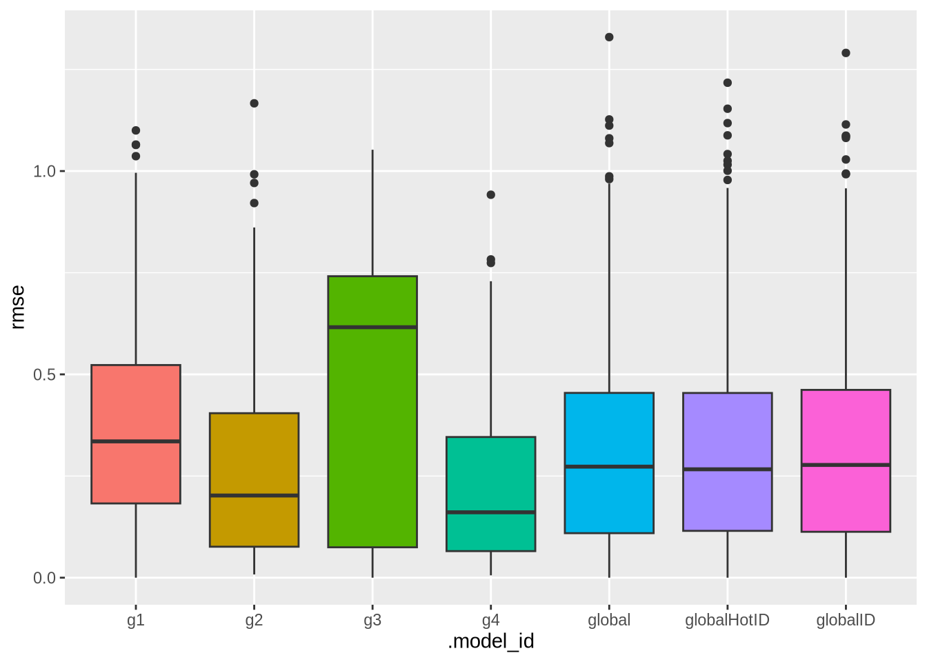
Breakdown
mun_names <- lookup_muni(code_muni = "all") %>%
  mutate(code_muni = substr(code_muni, 0, 6)) %>%
  mutate(name_muni = paste0(name_muni, ", ", abbrev_state)) %>%
  select(code_muni, name_muni)
Using year 2010models_accuracy %>%
left_join(mun_names, by = c("mun" = "code_muni")) %>%
select(.model_id, .model_desc, name_muni, rmse) %>%
mutate(rmse = round(rmse, 2)) %>%
arrange(.model_id, .model_desc, -rmse) %>%
datatable(filter = "top")# models_accuracy %>%
# left_join(mun_names, by = c("mun" = "code_muni")) %>%
# select(.model_id, .model_desc, name_muni, rmse) %>%
# mutate(rmse = round(rmse, 2)) %>%
# group_by(.model_desc) %>%
# mutate(.model_id = case_when(
# .model_id != "global" ~ "cluster",
# .default = .model_id
# )) %>%
# pivot_wider(names_from = .model_id, values_from = rmse) %>%
# mutate(dif = round(global - cluster, 2)) %>%
# ungroup() %>%
# datatable(filter = "top")# models_accuracy %>%
# left_join(mun_names, by = c("mun" = "code_muni")) %>%
# select(.model_id, .model_desc, name_muni, rmse) %>%
# group_by(.model_desc) %>%
# mutate(.model_id = case_when(
# .model_id != "global" ~ "cluster",
# .default = .model_id
# )) %>%
# pivot_wider(names_from = .model_id, values_from = rmse) %>%
# mutate(dif = round(global - cluster, 2)) %>%
# arrange(.model_desc, dif) %>%
# ggplot(aes(x = global, y = cluster, fill = .model_desc, color = dif)) +
# geom_point(size = 2, alpha = .3) +
# viridis::scale_color_viridis(option = "inferno") +
# theme_bw() +
# labs(x = "Global model", y = "Subset models", title = "RMSE error obtained with global and subset training strategies")Session info
sessionInfo()R version 4.3.2 (2023-10-31)
Platform: x86_64-conda-linux-gnu (64-bit)
Running under: CentOS Linux 7 (Core)
Matrix products: default
BLAS/LAPACK: /home/raphaelfs/miniconda3/envs/quarto/lib/libopenblasp-r0.3.25.so; LAPACK version 3.11.0
Random number generation:
RNG: L'Ecuyer-CMRG
Normal: Inversion
Sample: Rejection
locale:
[1] LC_CTYPE=pt_BR.UTF-8 LC_NUMERIC=C
[3] LC_TIME=pt_BR.UTF-8 LC_COLLATE=pt_BR.UTF-8
[5] LC_MONETARY=pt_BR.UTF-8 LC_MESSAGES=pt_BR.UTF-8
[7] LC_PAPER=pt_BR.UTF-8 LC_NAME=C
[9] LC_ADDRESS=C LC_TELEPHONE=C
[11] LC_MEASUREMENT=pt_BR.UTF-8 LC_IDENTIFICATION=C
time zone: America/Sao_Paulo
tzcode source: system (glibc)
attached base packages:
[1] stats graphics grDevices utils datasets methods base
other attached packages:
[1] rlang_1.1.1 ranger_0.16.0 sf_1.0-14 DT_0.28
[5] geobr_1.8.1 tictoc_1.2 kableExtra_1.3.4 dtwclust_5.5.12
[9] dtw_1.23-1 proxy_0.4-27 timetk_2.8.2 modeltime_1.2.5
[13] finetune_1.1.0 bonsai_0.2.1 yardstick_1.2.0 workflowsets_1.0.0
[17] workflows_1.1.3 tune_1.1.2 rsample_1.2.0 recipes_1.0.6
[21] parsnip_1.1.0 modeldata_1.1.0 infer_1.0.4 dials_1.2.0
[25] scales_1.2.1 broom_1.0.4 tidymodels_1.0.0 arrow_12.0.0
[29] lubridate_1.9.2 forcats_1.0.0 stringr_1.5.0 dplyr_1.1.2
[33] purrr_1.0.1 readr_2.1.4 tidyr_1.3.0 tibble_3.2.1
[37] ggplot2_3.4.2 tidyverse_2.0.0
loaded via a namespace (and not attached):
[1] rstudioapi_0.14 jsonlite_1.8.5 magrittr_2.0.3
[4] modeltools_0.2-23 farver_2.1.1 nloptr_2.0.3
[7] rmarkdown_2.22 vctrs_0.6.3 minqa_1.2.6
[10] webshot_0.5.4 htmltools_0.5.5 curl_5.0.2
[13] sass_0.4.6 parallelly_1.36.0 StanHeaders_2.26.26
[16] bslib_0.4.2 KernSmooth_2.23-21 htmlwidgets_1.6.2
[19] plyr_1.8.8 cachem_1.0.8 zoo_1.8-12
[22] mime_0.12 lifecycle_1.0.3 iterators_1.0.14
[25] pkgconfig_2.0.3 Matrix_1.5-4.1 R6_2.5.1
[28] fastmap_1.1.1 future_1.32.0 shiny_1.7.4
[31] clue_0.3-64 digest_0.6.31 colorspace_2.1-0
[34] furrr_0.3.1 RSpectra_0.16-1 crosstalk_1.2.0
[37] labeling_0.4.2 fansi_1.0.4 timechange_0.2.0
[40] httr_1.4.6 compiler_4.3.2 doParallel_1.0.17
[43] bit64_4.0.5 withr_2.5.0 backports_1.4.1
[46] DBI_1.1.3 MASS_7.3-60 lava_1.7.2.1
[49] classInt_0.4-9 units_0.8-2 tools_4.3.2
[52] httpuv_1.6.11 flexclust_1.4-1 future.apply_1.11.0
[55] nnet_7.3-19 glue_1.6.2 nlme_3.1-162
[58] promises_1.2.0.1 grid_4.3.2 cluster_2.1.4
[61] reshape2_1.4.4 generics_0.1.3 gtable_0.3.3
[64] tzdb_0.4.0 class_7.3-22 data.table_1.14.8
[67] hms_1.1.3 xml2_1.3.4 utf8_1.2.3
[70] ggrepel_0.9.3 foreach_1.5.2 pillar_1.9.0
[73] later_1.3.1 splines_4.3.2 lhs_1.1.6
[76] lattice_0.21-8 survival_3.5-5 bit_4.0.5
[79] tidyselect_1.2.0 knitr_1.43 svglite_2.1.1
[82] stats4_4.3.2 xfun_0.39 hardhat_1.3.0
[85] timeDate_4022.108 stringi_1.7.12 boot_1.3-28.1
[88] DiceDesign_1.9 yaml_2.3.7 evaluate_0.21
[91] codetools_0.2-19 cli_3.6.1 RcppParallel_5.1.7
[94] rpart_4.1.19 xtable_1.8-4 systemfonts_1.0.4
[97] jquerylib_0.1.4 munsell_0.5.0 Rcpp_1.0.10
[100] globals_0.16.2 parallel_4.3.2 ellipsis_0.3.2
[103] gower_1.0.1 assertthat_0.2.1 prettyunits_1.1.1
[106] lme4_1.1-35.1 GPfit_1.0-8 listenv_0.9.0
[109] viridisLite_0.4.2 ipred_0.9-13 e1071_1.7-13
[112] xts_0.13.1 prodlim_2019.11.13 rvest_1.0.3
[115] shinyjs_2.1.0