SBD clustering

Author

Raphael Saldanha

Last modification

December 1, 2023 | 09:07:18 +01:00

This notebooks aims to reproduce the metodology of the paper submitted to the SBD2023 conference, implementing the global and subset modelling.

This methodology aims to compare the perfomance of models trained with data from all municipalities time-series (global models) and models trained with subset of munipalities time-series (subset models).

Those subset will be created by a clustering algorithm considering the municipalities cases time-series.

Packages

library(tidyverse)
library(arrow)
library(tidymodels)
library(bonsai)
library(finetune)
library(modeltime)
library(timetk)
library(dtwclust)
library(kableExtra)
library(tictoc)
library(geobr)
library(DT)

Load data

tdengue <- read_parquet(file = "../tdengue.parquet") %>%
  drop_na() %>%
  select(mun, date, starts_with("cases"))

Note

NA values are created when the lagged variables were calculated. The rows containing those NA values are dropped due machine learning regressors constraints.
For validation purposes, only the cases and cases_lag* covariates variables are keep.

glimpse(tdengue)

Rows: 161,370
Columns: 9
$ mun        <chr> "110002", "110002", "110002", "110002", "110002", "110002",…
$ date       <date> 2011-02-06, 2011-02-13, 2011-02-20, 2011-02-27, 2011-03-06…
$ cases      <dbl> -0.51044592, 0.07880156, 0.66804904, 0.07880156, -0.5104459…
$ cases_lag1 <dbl> 2.43579149, -0.51044592, 0.07880156, 0.66804904, 0.07880156…
$ cases_lag2 <dbl> 0.66804904, 2.43579149, -0.51044592, 0.07880156, 0.66804904…
$ cases_lag3 <dbl> 0.07880156, 0.66804904, 2.43579149, -0.51044592, 0.07880156…
$ cases_lag4 <dbl> 0.66804904, 0.07880156, 0.66804904, 2.43579149, -0.51044592…
$ cases_lag5 <dbl> 0.66804904, 0.66804904, 0.07880156, 0.66804904, 2.43579149,…
$ cases_lag6 <dbl> -0.51044592, 0.66804904, 0.66804904, 0.07880156, 0.66804904…

Clustering

This procedure goal is to cluster the municipalities considering the cases time series similarities between them.

Prepare data

Prepare the data for use with the dtwclust package, pivoting the panel data to a wide format and matrix object.

cdengue <- tdengue %>%
  select(mun, date, cases) %>%
  mutate(mun = paste0("m_", mun)) %>%
  arrange(mun, date) %>%
  pivot_wider(names_from = mun, values_from = cases) %>%
  select(-date) %>%
  t() %>%
  tslist()

SBD method

The SBD method is used to cluster the municipalities, considering a shape-bases distance (k-Shape clustering algorithm) (Paparrizos and Gravano 2015).

326 municipalities will be clustered.

The clustering algorithm is applied with a varying number of \(k\) partitions from 3 to 8.

k_seq <- 3:8

tic()
clust <- tsclust(
  series = cdengue, 
  type = "partitional", 
  k = k_seq,
  distance = "sbd",
  seed = 123
)
toc()

0.257 sec elapsed

Cluster Validity Indices (CVI)

To choose the number of partitions, the Silhouette statistic is observed.

names(clust) <- paste0("k_", k_seq)
res_cvi <- sapply(clust, cvi, type = "internal") %>% 
  t() %>%
  as_tibble(rownames = "k") %>%
  arrange(-Sil)

res_cvi %>%
  kbl() %>%
  kable_styling()

k	Sil	SF	CH	DB	DBstar	D	COP
k_3	0.1747336	0.3501838	36.98758	2.260992	2.400068	0.0805315	0.3705055
k_4	0.1669509	0.2526978	34.15648	4.050796	4.597881	0.0676247	0.3688632
k_7	0.1625835	0.1135484	20.46483	2.802248	3.289527	0.0805315	0.3497498
k_8	0.1294623	0.1012342	20.25096	1.906407	2.268955	0.0660755	0.3456895
k_6	0.0914225	0.1541329	29.42529	4.230747	7.206356	0.0280277	0.3317256
k_5	0.0517861	0.1915811	27.11958	3.855824	5.374118	0.0353306	0.3523987

Select cluster with higher Silhouette statistic

sel_clust <- clust[[res_cvi[[1,1]]]]

plot(sel_clust)

Cluster sizes

table(sel_clust@cluster)


  1   2   3 
 34 251  41

Identify municipalities and cluster id

Finally, the cluster partition ID is added to the main dataset.

cluster_ids <- tibble(
  mun = names(cdengue) %>% substr(3, 9),
  group = as.character(sel_clust@cluster)
)

tdengue <- left_join(tdengue, cluster_ids, by = "mun")

Train and test split

Split the data into training and testing. The function time_series_split handles the time series, not shuffling them, and considering the panel data format, as depicted in the message about overlapping timestamps detected.

The last two years data will be used as the training set.

tdengue_split <- tdengue %>%
  time_series_split(
    date_var = date, 
    assess = 52*2,
    cumulative = TRUE
  )

Data is not ordered by the 'date_var'. Resamples will be arranged by `date`.

Overlapping Timestamps Detected. Processing overlapping time series together using sliding windows.

tdengue_split

<Analysis/Assess/Total>
<127466/33904/161370>

K-folds

The training set will be split into k folds.

tdengue_split_folds <- training(tdengue_split) %>%
  vfold_cv(v = 5)

Recipes

The global and subset models training specification are called recipes. The procedure bellow creates a list of those recipes.

recipes_list <- list()

Global

The global training recipe uses data from all municipalities for training the models.

The date and group variables are removed prior training
The municipality identification variable is treated as an Id variable, taking no place as a predictor in the training process

recipe_global <- recipe(cases ~ ., data = training(tdengue_split)) %>%
  step_rm(date, group) %>%
  update_role(mun, new_role = "id variable")

recipes_list <- append(recipes_list, list(global = recipe_global))

rm(recipe_global)

Groups

For each group created by the clustering process, a specific training recipe will be created. For this, the first step is to filter rows from the training set, keep only the rows belonging to the group in the loop
The date and group variables are removed prior training
The municipality identification variable is treated as an Id variable, taking no place as a predictor in the training process

for(g in unique(tdengue$group)){
  tmp <- recipe(cases ~ ., data = training(tdengue_split)) %>%
    step_filter(group == !!g) %>%
    step_rm(date, group) %>%
    update_role(mun, new_role = "id variable")
  
  tmp <- list(tmp)
  tmp <- setNames(tmp, paste0("g", g))
  
  recipes_list <- append(recipes_list, tmp)
  
  rm(tmp)
}

Regressors specification

Random forest

A Random Forest specification using the ranger engine. The trees and min_n hyperparameters will be tuned.

rf_spec <- rand_forest(
  trees = tune(),
  min_n = tune()
) %>%
  set_engine("ranger") %>%
  set_mode("regression")

LightGBM

# lgbm_spec <- boost_tree(
#   trees = tune(),
#   min_n = tune(),
#   tree_depth = tune()
# ) %>%
#   set_engine("lightgbm") %>%
#   set_mode("regression")

Workflow set

This step creates a workflow set, combining the training recipes and regressors specifications.

all_workflows <- workflow_set(
  preproc = recipes_list, 
  models = list(rf = rf_spec), 
  cross = TRUE
)

Tune

This step tunes the training hyperparameters of each workflow.

doParallel::registerDoParallel()

tic()
race_results <- 
  all_workflows %>%
  workflow_map(
    "tune_race_anova",
    seed = 345,
    resamples = tdengue_split_folds,
    grid = 10,
    control = control_race(parallel_over = "everything"),
    verbose = TRUE
  )

i 1 of 4 tuning:     global_rf

Warning in mclapply(argsList, FUN, mc.preschedule = preschedule, mc.set.seed =
set.seed, : scheduled core 5 did not deliver a result, all values of the job
will be affected

✔ 1 of 4 tuning:     global_rf (25m 1.5s)

i 2 of 4 tuning:     g3_rf

✔ 2 of 4 tuning:     g3_rf (2m 24s)

i 3 of 4 tuning:     g1_rf

✔ 3 of 4 tuning:     g1_rf (1m 19.9s)

i 4 of 4 tuning:     g2_rf

✔ 4 of 4 tuning:     g2_rf (18m 47.6s)

toc()

2853.792 sec elapsed

Fit

Each workflow will be trained using the tuned hyperparameters, considering the RMSE metric as reference.

This procedure creates a list of trained models, containing the fit results and a list of the municipalities used on the training of each workflow.

The global workflow is trained with data from all municipalities and the subsets workflows are trained using the respective municipalities list given by the cluster algorithm.

tic()
trained_models <- list()
for(w in unique(race_results$wflow_id)){
  best_tune <- race_results %>%
    extract_workflow_set_result(w) %>%
    select_best("rmse")
  
  final_fit <- race_results %>%
    extract_workflow(w) %>%
    finalize_workflow(best_tune) %>%
    fit(training(tdengue_split))
  
  mold <- extract_mold(final_fit)
  train_ids <- mold$extras$roles$`id variable` %>%
    distinct() %>%
    pull() %>%
    as.character()
  
  final_fit <- list(
    list(
      "final_fit" = final_fit, 
      "train_ids" = train_ids
    )
  )
  
  final_fit <- setNames(final_fit, paste0(w))
  
  trained_models <- append(trained_models, final_fit)
}
toc()

369.351 sec elapsed

Accuracy

After training each workflow, the accuracy of the models are obtained applying the fitted models on the testing set.

For the global model, all municipalities are using for testing. For the subsets models, only data from the subset’s municipalities are considered for testing.

The RMSE metric is obtained for each workflow and municipality.

models_accuracy <- tibble()
for(t in 1:length(trained_models)){
  
  model_tbl <- modeltime_table(trained_models[[t]][[1]]) 
  testing_set <- testing(tdengue_split) %>%
    filter(mun %in% trained_models[[t]][[2]])
  

  calib_tbl <- model_tbl %>%
      modeltime_calibrate(
        new_data = testing_set, 
        id       = "mun"
      )
  
  res <- calib_tbl %>% 
      modeltime_accuracy(
        acc_by_id = TRUE, 
        metric_set = metric_set(rmse)
      )
  
  res$.model_id <- word(names(trained_models[t]), 1, sep = "_")
  
  models_accuracy <- bind_rows(models_accuracy, res)
}

This plot presents the RMSE distribution across the workflows.

ggplot(data = models_accuracy, aes(x = .model_id, y = rmse, fill = .model_desc)) +
  geom_boxplot()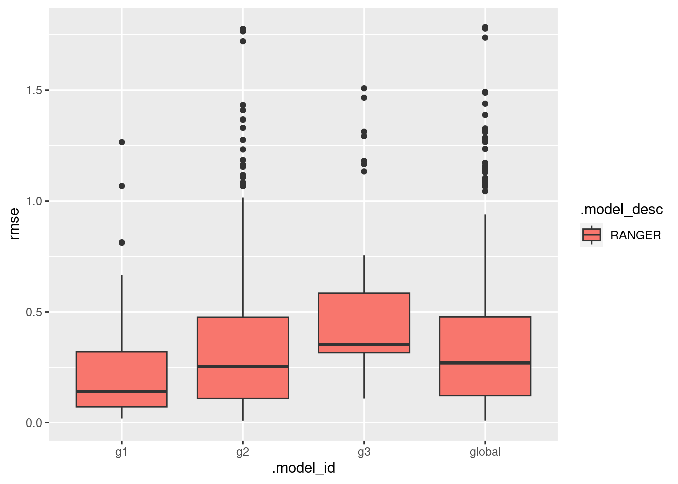

Breakdown

mun_names <- lookup_muni(code_muni = "all") %>%
  mutate(code_muni = substr(code_muni, 0, 6)) %>%
  mutate(name_muni = paste0(name_muni, ", ", abbrev_state)) %>%
  select(code_muni, name_muni)

Using year 2010

models_accuracy %>% 
  left_join(mun_names, by = c("mun" = "code_muni")) %>%
  select(.model_id, .model_desc, name_muni, rmse) %>%
  mutate(rmse = round(rmse, 2)) %>%
  arrange(.model_id, .model_desc, -rmse) %>%
  datatable(filter = "top")

models_accuracy %>% 
  left_join(mun_names, by = c("mun" = "code_muni")) %>%
  select(.model_id, .model_desc, name_muni, rmse) %>%
  mutate(rmse = round(rmse, 2)) %>%
  group_by(.model_desc) %>%
  mutate(.model_id = case_when(
    .model_id != "global" ~ "cluster",
    .default = .model_id
  )) %>%
  pivot_wider(names_from = .model_id, values_from = rmse) %>%
  mutate(dif = round(global - cluster, 2)) %>% 
  ungroup() %>%
  datatable(filter = "top")

models_accuracy %>% 
  left_join(mun_names, by = c("mun" = "code_muni")) %>%
  select(.model_id, .model_desc, name_muni, rmse) %>%
  group_by(.model_desc) %>%
  mutate(.model_id = case_when(
    .model_id != "global" ~ "cluster",
    .default = .model_id
  )) %>%
  pivot_wider(names_from = .model_id, values_from = rmse) %>%
  mutate(dif = round(global - cluster, 2)) %>% 
  arrange(.model_desc, dif) %>%
  ggplot(aes(x = global, y = cluster, fill = .model_desc, color = dif)) +
  geom_point(size = 2, alpha = .3) +
  viridis::scale_color_viridis(option = "inferno") +
  theme_bw() +
  labs(x = "Global model", y = "Subset models", title = "RMSE error obtained with global and subset training strategies")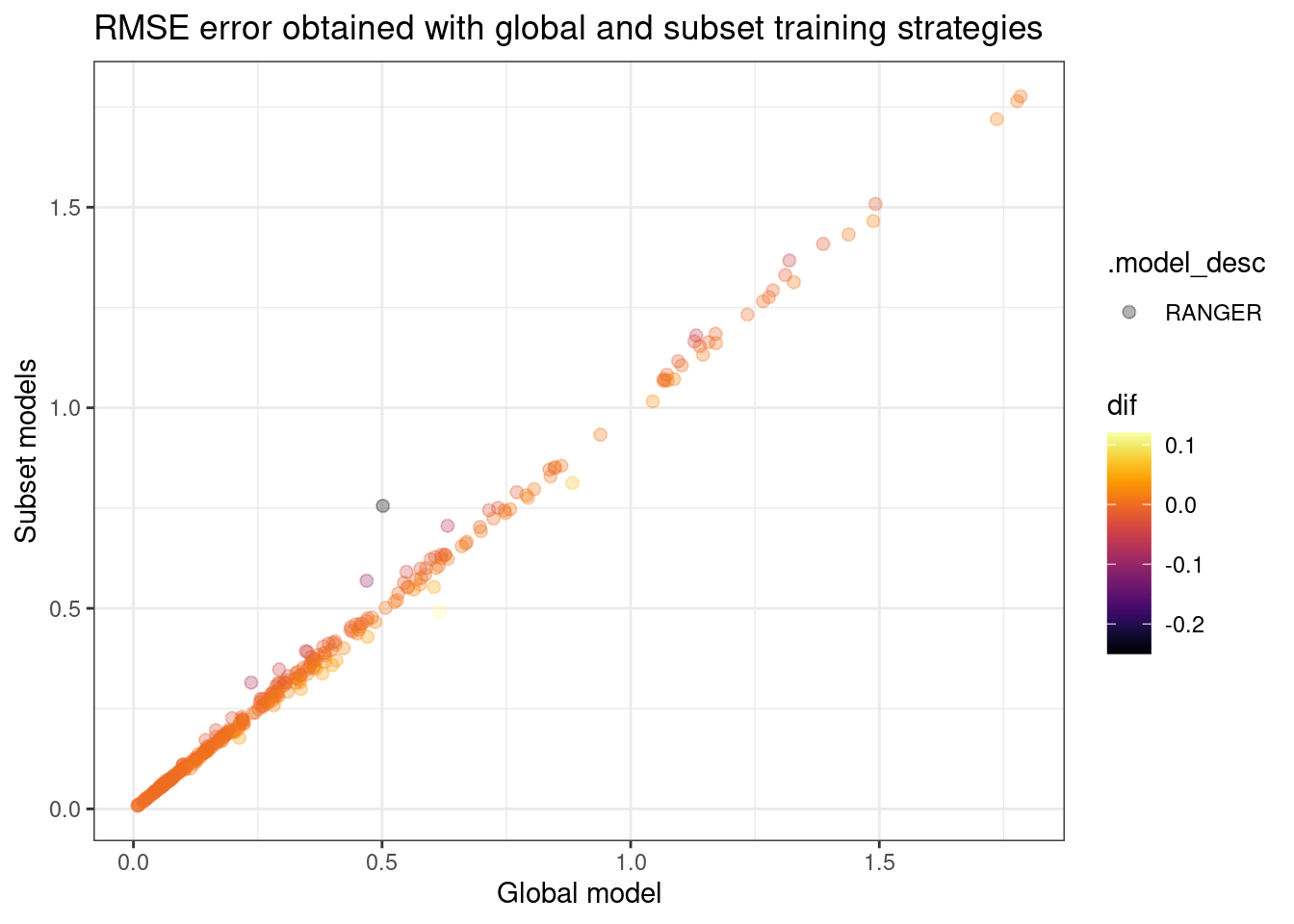

Session info

sessionInfo()

R version 4.1.2 (2021-11-01)
Platform: x86_64-pc-linux-gnu (64-bit)
Running under: Ubuntu 22.04.2 LTS

Matrix products: default
BLAS:   /usr/lib/x86_64-linux-gnu/blas/libblas.so.3.10.0
LAPACK: /usr/lib/x86_64-linux-gnu/lapack/liblapack.so.3.10.0

Random number generation:
 RNG:     L'Ecuyer-CMRG 
 Normal:  Inversion 
 Sample:  Rejection 
 
locale:
 [1] LC_CTYPE=pt_BR.UTF-8       LC_NUMERIC=C              
 [3] LC_TIME=en_US.UTF-8        LC_COLLATE=en_US.UTF-8    
 [5] LC_MONETARY=en_US.UTF-8    LC_MESSAGES=en_US.UTF-8   
 [7] LC_PAPER=en_US.UTF-8       LC_NAME=C                 
 [9] LC_ADDRESS=C               LC_TELEPHONE=C            
[11] LC_MEASUREMENT=en_US.UTF-8 LC_IDENTIFICATION=C       

attached base packages:
[1] stats     graphics  grDevices utils     datasets  methods   base     

other attached packages:
 [1] rlang_1.1.1        ranger_0.15.1      DT_0.28            geobr_1.7.0       
 [5] tictoc_1.2         kableExtra_1.3.4   dtwclust_5.5.12    dtw_1.23-1        
 [9] proxy_0.4-27       timetk_2.8.3       modeltime_1.2.7    finetune_1.1.0    
[13] bonsai_0.2.1       yardstick_1.2.0    workflowsets_1.0.1 workflows_1.1.3   
[17] tune_1.1.1         rsample_1.1.1      recipes_1.0.6      parsnip_1.1.0     
[21] modeldata_1.1.0    infer_1.0.4        dials_1.2.0        scales_1.2.1      
[25] broom_1.0.5        tidymodels_1.1.0   arrow_12.0.1.1     lubridate_1.9.2   
[29] forcats_1.0.0      stringr_1.5.0      dplyr_1.1.2        purrr_1.0.1       
[33] readr_2.1.4        tidyr_1.3.0        tibble_3.2.1       ggplot2_3.4.2     
[37] tidyverse_2.0.0   

loaded via a namespace (and not attached):
  [1] backports_1.4.1     systemfonts_1.0.4   plyr_1.8.8         
  [4] splines_4.1.2       crosstalk_1.2.0     listenv_0.9.0      
  [7] digest_0.6.33       foreach_1.5.2       htmltools_0.5.5    
 [10] viridis_0.6.3       fansi_1.0.4         magrittr_2.0.3     
 [13] doParallel_1.0.17   cluster_2.1.2       tzdb_0.4.0         
 [16] globals_0.16.2      gower_1.0.1         RcppParallel_5.1.7 
 [19] xts_0.13.1          svglite_2.1.1       hardhat_1.3.0      
 [22] timechange_0.2.0    prettyunits_1.1.1   colorspace_2.1-0   
 [25] rvest_1.0.3         ggrepel_0.9.3       xfun_0.39          
 [28] jsonlite_1.8.7      lme4_1.1-34         survival_3.2-13    
 [31] zoo_1.8-12          iterators_1.0.14    glue_1.6.2         
 [34] gtable_0.3.3        ipred_0.9-14        webshot_0.5.5      
 [37] future.apply_1.11.0 DBI_1.1.3           Rcpp_1.0.11        
 [40] viridisLite_0.4.2   xtable_1.8-4        units_0.8-2        
 [43] clue_0.3-64         GPfit_1.0-8         bit_4.0.5          
 [46] stats4_4.1.2        lava_1.7.2.1        StanHeaders_2.26.27
 [49] prodlim_2023.03.31  htmlwidgets_1.6.2   httr_1.4.6         
 [52] modeltools_0.2-23   ellipsis_0.3.2      farver_2.1.1       
 [55] pkgconfig_2.0.3     sass_0.4.7          nnet_7.3-17        
 [58] utf8_1.2.3          labeling_0.4.2      tidyselect_1.2.0   
 [61] DiceDesign_1.9      reshape2_1.4.4      later_1.3.1        
 [64] cachem_1.0.8        munsell_0.5.0       tools_4.1.2        
 [67] cli_3.6.1           generics_0.1.3      evaluate_0.21      
 [70] fastmap_1.1.1       yaml_2.3.7          knitr_1.43         
 [73] bit64_4.0.5         nlme_3.1-155        future_1.33.0      
 [76] mime_0.12           xml2_1.3.5          flexclust_1.4-1    
 [79] compiler_4.1.2      rstudioapi_0.15.0   curl_5.0.1         
 [82] e1071_1.7-13        lhs_1.1.6           bslib_0.5.0        
 [85] stringi_1.7.12      highr_0.10          RSpectra_0.16-1    
 [88] lattice_0.20-45     Matrix_1.6-0        nloptr_2.0.3       
 [91] classInt_0.4-9      shinyjs_2.1.0       vctrs_0.6.3        
 [94] pillar_1.9.0        lifecycle_1.0.3     furrr_0.3.1        
 [97] jquerylib_0.1.4     data.table_1.14.8   httpuv_1.6.11      
[100] R6_2.5.1            promises_1.2.0.1    gridExtra_2.3      
[103] KernSmooth_2.23-20  parallelly_1.36.0   codetools_0.2-18   
[106] boot_1.3-28         MASS_7.3-55         assertthat_0.2.1   
[109] withr_2.5.0         parallel_4.1.2      hms_1.1.3          
[112] grid_4.1.2          rpart_4.1.16        timeDate_4022.108  
[115] minqa_1.2.5         class_7.3-20        rmarkdown_2.23     
[118] sf_1.0-14           shiny_1.7.4.1

References

Paparrizos, John, and Luis Gravano. 2015. “K-Shape.” Proceedings of the 2015 ACM SIGMOD International Conference on Management of Data, May. https://doi.org/10.1145/2723372.2737793.