Scaled cases, cumulative

Author

Raphael Saldanha

Last modification

December 1, 2023 | 09:07:18 +01:00

This notebook aims to cluster the Brazilian municipalities considering scaled (standardized) dengue cases time-series similarities.

Packages

library(tidyverse)
library(lubridate)
library(arrow)
library(timetk)
library(dtwclust)
library(kableExtra)
library(tictoc)
source("../functions.R")

Load data

Load the aggregated data.

tdengue <- open_dataset(sources = data_dir("bundled_data/tdengue.parquet")) %>%
    select(mun, date, cases = cases_cum) %>%
    collect()

dim(tdengue)

[1] 340179      3

Prepare data

The chunk bellow executes various steps to prepare the data for clustering.

tdengue <- tdengue %>%
  # Prepare time series
  mutate(mun = paste0("m_", mun)) %>%
  arrange(mun, date) %>%
  pivot_wider(names_from = mun, values_from = cases) %>%
  select(-date) %>%
  t() %>%
  tslist()

saveRDS(object = tdengue, file = "tdengue.rds")

length(tdengue)

[1] 679

Clustering

Sequence of k groups to be used.

k_seq <- 2:10

DTW (basic)

tic()
clust_dtw <- tsclust(
  series = tdengue, 
  type = "partitional", 
  k = k_seq,
  distance = "dtw_basic",
  seed = 13
)
toc()

39.132 sec elapsed

names(clust_dtw) <- paste0("k_", k_seq)
res_cvi <- sapply(clust_dtw, cvi, type = "internal") %>% 
  t() %>%
  as_tibble(rownames = "k") %>%
  arrange(-Sil)

res_cvi %>%
  gt::gt()

k	Sil	CH	DB	DBstar	D	COP
k_2	0.3883485	219.03946	1.134304	1.134304	0.008077949	0.15430130
k_3	0.3067752	310.90157	1.635604	1.775981	0.006456940	0.12341630
k_5	0.2387272	162.71153	1.759704	2.280500	0.006971102	0.09710109
k_8	0.2052530	116.02794	1.497911	2.157663	0.010105561	0.08426017
k_9	0.1759150	110.48283	1.982305	3.102040	0.007701467	0.07432019
k_7	0.1677298	116.57366	1.604325	2.207429	0.010855206	0.08933756
k_10	0.1586523	80.28211	2.273564	3.023525	0.006111798	0.08597771
k_4	0.1539778	147.65699	2.473204	3.436038	0.005005953	0.12329358
k_6	0.1527731	126.08954	2.013522	2.576196	0.005165569	0.10876459

sel_clust <- clust_dtw[[res_cvi[[1,1]]]]

plot(sel_clust)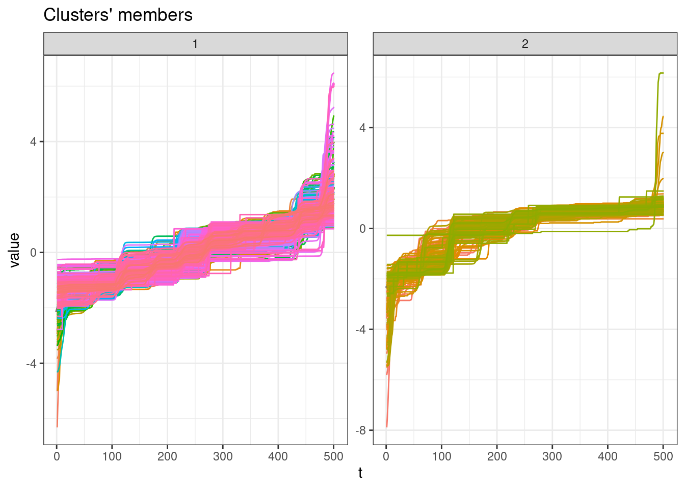

plot(sel_clust, type = "centroids", lty = 1)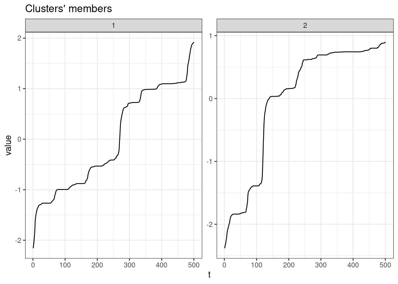

table(sel_clust@cluster)


  1   2 
551 128

Soft-DTW

tic()
clust_sdtw <- tsclust(
  series = tdengue, 
  type = "partitional", 
  k = k_seq,
  distance = "sdtw",
  seed = 13
)
toc()

193.822 sec elapsed

names(clust_sdtw) <- paste0("k_", k_seq)
res_cvi <- sapply(clust_sdtw, cvi, type = "internal") %>% 
  t() %>%
  as_tibble(rownames = "k") %>%
  arrange(-Sil)

res_cvi %>%
  gt::gt()

k	Sil	SF	CH	DB	DBstar	D	COP
k_9	4.6835404	3.301961e-04	-1198.16808	0.4328621	70.9687638	-0.027622202	-0.001783289
k_3	0.5874870	1.210092e-08	241.76435	0.4728893	0.6095286	-0.016428914	0.017947639
k_2	0.5526841	1.864919e-08	-157.74645	0.6603416	0.6603416	-0.008343487	0.076892143
k_7	0.5143244	2.926145e-06	1776.33826	3.5865645	-11.8749979	-0.024224946	0.003868853
k_6	0.5091103	4.869410e-04	463.73188	2.1072188	0.3291628	-0.018669198	0.005947036
k_10	0.4865815	8.516047e-01	1744.16238	2.2000345	-13.7430978	-0.020388668	0.003773382
k_5	0.4759798	3.530744e-08	219.42676	1.0472748	2.8079291	-0.015917823	0.007728450
k_4	0.2085165	1.043811e-05	46.69006	1.5530459	-0.6703440	-0.016278775	0.027708772
k_8	0.0811271	1.595867e-05	51191.47920	3.6371109	-5.0907762	-0.024336278	0.001610495

sel_clust <- clust_sdtw[[res_cvi[[1,1]]]]

plot(sel_clust)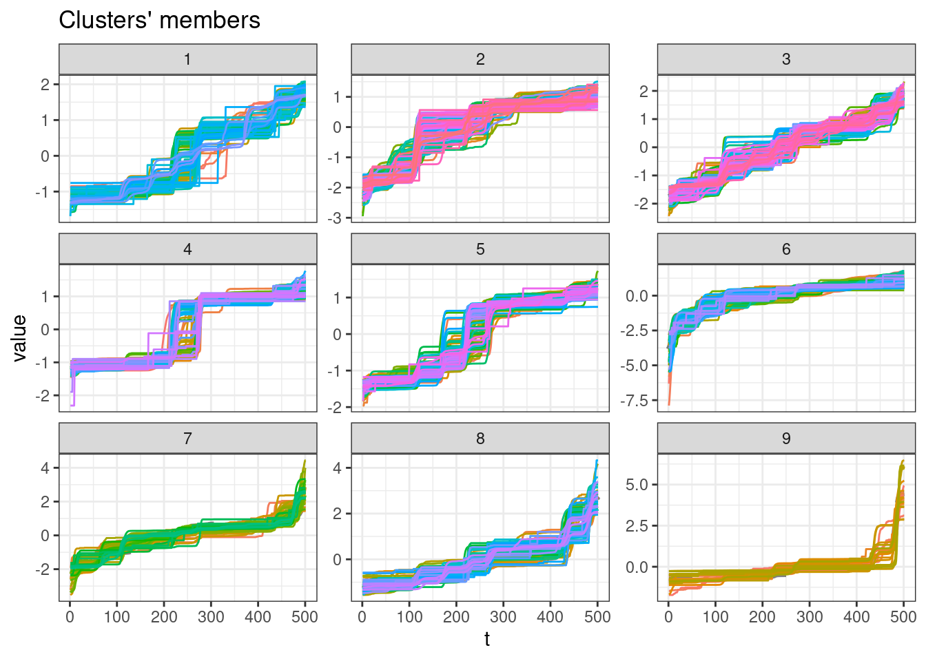

plot(sel_clust, type = "centroids", lty = 1)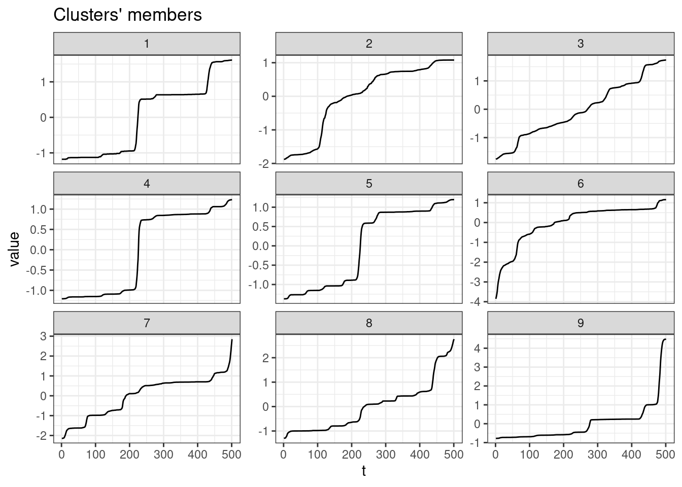

table(sel_clust@cluster)


  1   2   3   4   5   6   7   8   9 
 74 106 102  83  89  78  44  81  22

cluster_ids <- tibble(
  mun = names(tdengue) %>% substr(3, 9),
  group = as.character(sel_clust@cluster)
) 

saveRDS(object = cluster_ids, file = "clust_sdtw_ids.rds")

SBD

tic()
clust_sbd <- tsclust(
  series = tdengue, 
  type = "partitional", 
  k = k_seq,
  distance = "sbd",
  seed = 13
)
toc()

0.756 sec elapsed

names(clust_sbd) <- paste0("k_", k_seq)
res_cvi <- sapply(clust_sbd, cvi, type = "internal") %>% 
  t() %>%
  as_tibble(rownames = "k") %>%
  arrange(-Sil)

res_cvi %>%
  gt::gt()

k	Sil	SF	CH	DB	DBstar	D	COP
k_2	0.4442625	0.5940473	345.3780	1.035863	1.035863	0.008004787	0.20201102
k_3	0.4022197	0.5792206	346.5557	1.239092	1.387231	0.001858214	0.12732693
k_4	0.3334983	0.5737804	245.6445	1.121578	1.815766	0.002032385	0.10409579
k_7	0.3274548	0.5339155	190.7100	1.212410	2.079583	0.004857007	0.06826826
k_6	0.3125595	0.5426452	206.1180	1.239948	2.105174	0.008653764	0.07328745
k_10	0.2993463	0.5225233	168.3385	1.828146	3.486689	0.002307383	0.05626920
k_9	0.2813463	0.5244313	182.8368	1.213397	1.947885	0.002827627	0.05685390
k_5	0.2604179	0.5603160	209.0601	1.290158	1.825457	0.003340171	0.10155246
k_8	0.1947688	0.5344965	148.8106	1.642704	3.682444	0.002371686	0.07799687

sel_clust <- clust_sbd[[res_cvi[[1,1]]]]

plot(sel_clust)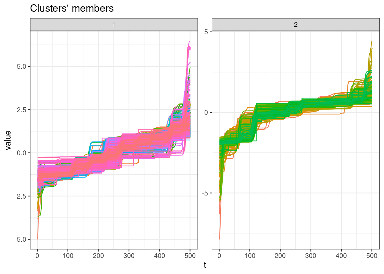

plot(sel_clust, type = "centroids", lty = 1)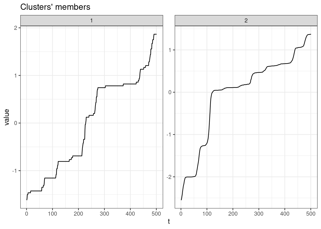

table(sel_clust@cluster)


  1   2 
500 179

GAK

tic()
clust_gak <- tsclust(
  series = tdengue, 
  type = "partitional", 
  k = k_seq,
  distance = "gak",
  seed = 13
)
toc()

280.382 sec elapsed

names(clust_gak) <- paste0("k_", k_seq)
res_cvi <- sapply(clust_gak, cvi, type = "internal") %>% 
  t() %>%
  as_tibble(rownames = "k") %>%
  arrange(-Sil)

res_cvi %>%
  gt::gt()

k	Sil	SF	CH	DB	DBstar	D	COP
k_2	0.4703437	0.6318950	346.9030	0.7492626	0.7492626	0.002673344	0.22610650
k_3	0.4242503	0.6317923	350.9145	1.1578518	1.3150938	0.001689423	0.12032277
k_4	0.3404306	0.6317602	248.3140	1.0644928	1.7873944	0.001860028	0.09770063
k_7	0.3391378	0.6315128	204.6923	1.2022774	2.0564247	0.003583292	0.06365358
k_6	0.3320730	0.6315865	228.3494	1.1336897	1.8636779	0.004311562	0.06847479
k_9	0.3173288	0.6314596	178.8928	1.1311449	1.9720656	0.004519858	0.04981730
k_10	0.3094439	0.6314500	177.1258	1.7581411	3.6257840	0.001690421	0.05150554
k_5	0.2528416	0.6316542	190.1814	1.5612030	2.0839318	0.001970852	0.09056517
k_8	0.2169763	0.6315151	152.0770	1.7145901	4.1675547	0.001897451	0.07208410

sel_clust <- clust_gak[[res_cvi[[1,1]]]]

plot(sel_clust)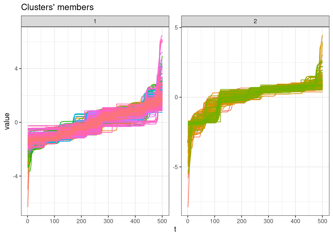

plot(sel_clust, type = "centroids", lty = 1)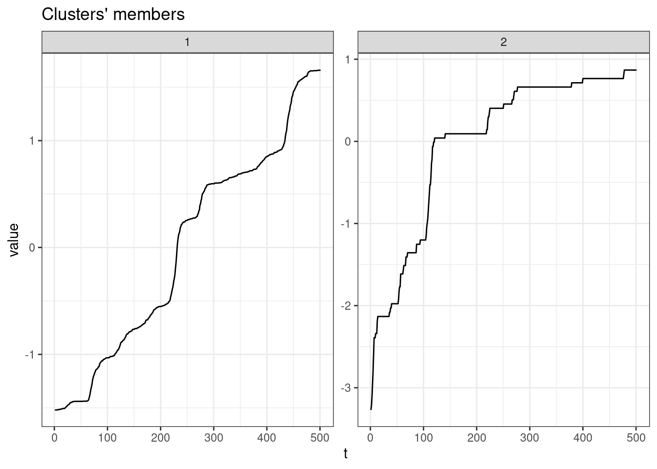

table(sel_clust@cluster)


  1   2 
535 144

Session info

sessionInfo()

R version 4.3.2 (2023-10-31)
Platform: x86_64-pc-linux-gnu (64-bit)
Running under: Ubuntu 22.04.3 LTS

Matrix products: default
BLAS:   /usr/lib/x86_64-linux-gnu/blas/libblas.so.3.10.0 
LAPACK: /usr/lib/x86_64-linux-gnu/lapack/liblapack.so.3.10.0

Random number generation:
 RNG:     L'Ecuyer-CMRG 
 Normal:  Inversion 
 Sample:  Rejection 
 
locale:
 [1] LC_CTYPE=en_US.UTF-8       LC_NUMERIC=C              
 [3] LC_TIME=en_CA.UTF-8        LC_COLLATE=en_US.UTF-8    
 [5] LC_MONETARY=en_CA.UTF-8    LC_MESSAGES=en_US.UTF-8   
 [7] LC_PAPER=en_CA.UTF-8       LC_NAME=C                 
 [9] LC_ADDRESS=C               LC_TELEPHONE=C            
[11] LC_MEASUREMENT=en_CA.UTF-8 LC_IDENTIFICATION=C       

time zone: Europe/Paris
tzcode source: system (glibc)

attached base packages:
[1] stats     graphics  grDevices utils     datasets  methods   base     

other attached packages:
 [1] tictoc_1.2       kableExtra_1.3.4 dtwclust_5.5.12  dtw_1.23-1      
 [5] proxy_0.4-27     timetk_2.9.0     arrow_13.0.0.1   lubridate_1.9.3 
 [9] forcats_1.0.0    stringr_1.5.0    dplyr_1.1.3      purrr_1.0.2     
[13] readr_2.1.4      tidyr_1.3.0      tibble_3.2.1     ggplot2_3.4.4   
[17] tidyverse_2.0.0 

loaded via a namespace (and not attached):
  [1] rlang_1.1.2         magrittr_2.0.3      clue_0.3-65        
  [4] furrr_0.3.1         flexclust_1.4-1     compiler_4.3.2     
  [7] systemfonts_1.0.5   vctrs_0.6.4         reshape2_1.4.4     
 [10] rvest_1.0.3         lhs_1.1.6           tune_1.1.2         
 [13] pkgconfig_2.0.3     fastmap_1.1.1       ellipsis_0.3.2     
 [16] labeling_0.4.3      utf8_1.2.4          promises_1.2.1     
 [19] rmarkdown_2.25      prodlim_2023.08.28  tzdb_0.4.0         
 [22] bit_4.0.5           xfun_0.41           modeltools_0.2-23  
 [25] jsonlite_1.8.7      recipes_1.0.8       later_1.3.1        
 [28] parallel_4.3.2      cluster_2.1.4       R6_2.5.1           
 [31] stringi_1.7.12      rsample_1.2.0       parallelly_1.36.0  
 [34] rpart_4.1.21        Rcpp_1.0.11         assertthat_0.2.1   
 [37] dials_1.2.0         iterators_1.0.14    knitr_1.45         
 [40] future.apply_1.11.0 zoo_1.8-12          httpuv_1.6.12      
 [43] Matrix_1.6-1.1      splines_4.3.2       nnet_7.3-19        
 [46] timechange_0.2.0    tidyselect_1.2.0    rstudioapi_0.15.0  
 [49] yaml_2.3.7          timeDate_4022.108   codetools_0.2-19   
 [52] listenv_0.9.0       lattice_0.22-5      plyr_1.8.9         
 [55] shiny_1.7.5.1       withr_2.5.2         evaluate_0.23      
 [58] future_1.33.0       survival_3.5-7      RcppParallel_5.1.7 
 [61] xml2_1.3.5          xts_0.13.1          pillar_1.9.0       
 [64] foreach_1.5.2       stats4_4.3.2        shinyjs_2.1.0      
 [67] generics_0.1.3      hms_1.1.3           munsell_0.5.0      
 [70] scales_1.2.1        xtable_1.8-4        globals_0.16.2     
 [73] class_7.3-22        glue_1.6.2          tools_4.3.2        
 [76] data.table_1.14.8   RSpectra_0.16-1     webshot_0.5.5      
 [79] gower_1.0.1         grid_4.3.2          yardstick_1.2.0    
 [82] ipred_0.9-14        colorspace_2.1-0    cli_3.6.1          
 [85] DiceDesign_1.9      workflows_1.1.3     parsnip_1.1.1      
 [88] fansi_1.0.5         viridisLite_0.4.2   gt_0.10.0          
 [91] svglite_2.1.2       lava_1.7.3          gtable_0.3.4       
 [94] GPfit_1.0-8         sass_0.4.7          digest_0.6.33      
 [97] ggrepel_0.9.4       farver_2.1.1        htmlwidgets_1.6.2  
[100] htmltools_0.5.7     lifecycle_1.0.4     httr_1.4.7         
[103] hardhat_1.3.0       mime_0.12           bit64_4.0.5        
[106] MASS_7.3-60