Scaled cases

Author

Raphael Saldanha

Last modification

December 1, 2023 | 09:07:18 +01:00

This notebook aims to cluster the Brazilian municipalities considering scaled (standardized) dengue cases time-series similarities.

Packages

library(tidyverse)
library(lubridate)
library(arrow)
library(timetk)
library(dtwclust)
library(kableExtra)
library(tictoc)
source("../functions.R")

Load data

Load the aggregated data.

tdengue <- open_dataset(sources = data_dir("bundled_data/tdengue.parquet")) %>%
    select(mun, date, cases) %>%
    collect()

dim(tdengue)

[1] 340179      3

Prepare data

The chunk bellow executes various steps to prepare the data for clustering.

tdengue <- tdengue %>%
  # Prepare time series
  mutate(mun = paste0("m_", mun)) %>%
  arrange(mun, date) %>%
  pivot_wider(names_from = mun, values_from = cases) %>%
  select(-date) %>%
  t() %>%
  tslist()

length(tdengue)

[1] 679

Clustering

Sequence of k groups to be used.

k_seq <- 2:10

DTW (basic)

tic()
clust_dtw <- tsclust(
  series = tdengue, 
  type = "partitional", 
  k = k_seq,
  distance = "dtw_basic",
  seed = 13
)
toc()

44.727 sec elapsed

names(clust_dtw) <- paste0("k_", k_seq)
res_cvi <- sapply(clust_dtw, cvi, type = "internal") %>% 
  t() %>%
  as_tibble(rownames = "k") %>%
  arrange(-Sil)

res_cvi %>%
  gt::gt()

k	Sil	CH	DB	DBstar	D	COP
k_2	0.22470565	471.19772	2.169633	2.169633	0.09802846	0.4465088
k_6	0.16590632	129.12898	1.492001	1.779535	0.08842332	0.3564468
k_5	0.12371981	166.97238	1.873249	2.231609	0.08368662	0.3581035
k_3	0.12269031	282.64604	2.352913	2.754531	0.08676909	0.4086315
k_4	0.11888356	193.62938	1.898608	2.232433	0.08471016	0.3694141
k_10	0.10437071	82.16793	1.872270	2.348246	0.10197290	0.3198181
k_7	0.07891310	105.14468	2.366061	2.737811	0.10021368	0.3467224
k_9	0.05778652	87.10300	1.950026	2.716834	0.10021368	0.3233407
k_8	0.05494472	100.42993	1.902694	2.559555	0.07642521	0.3449551

sel_clust <- clust_dtw[[res_cvi[[1,1]]]]

plot(sel_clust)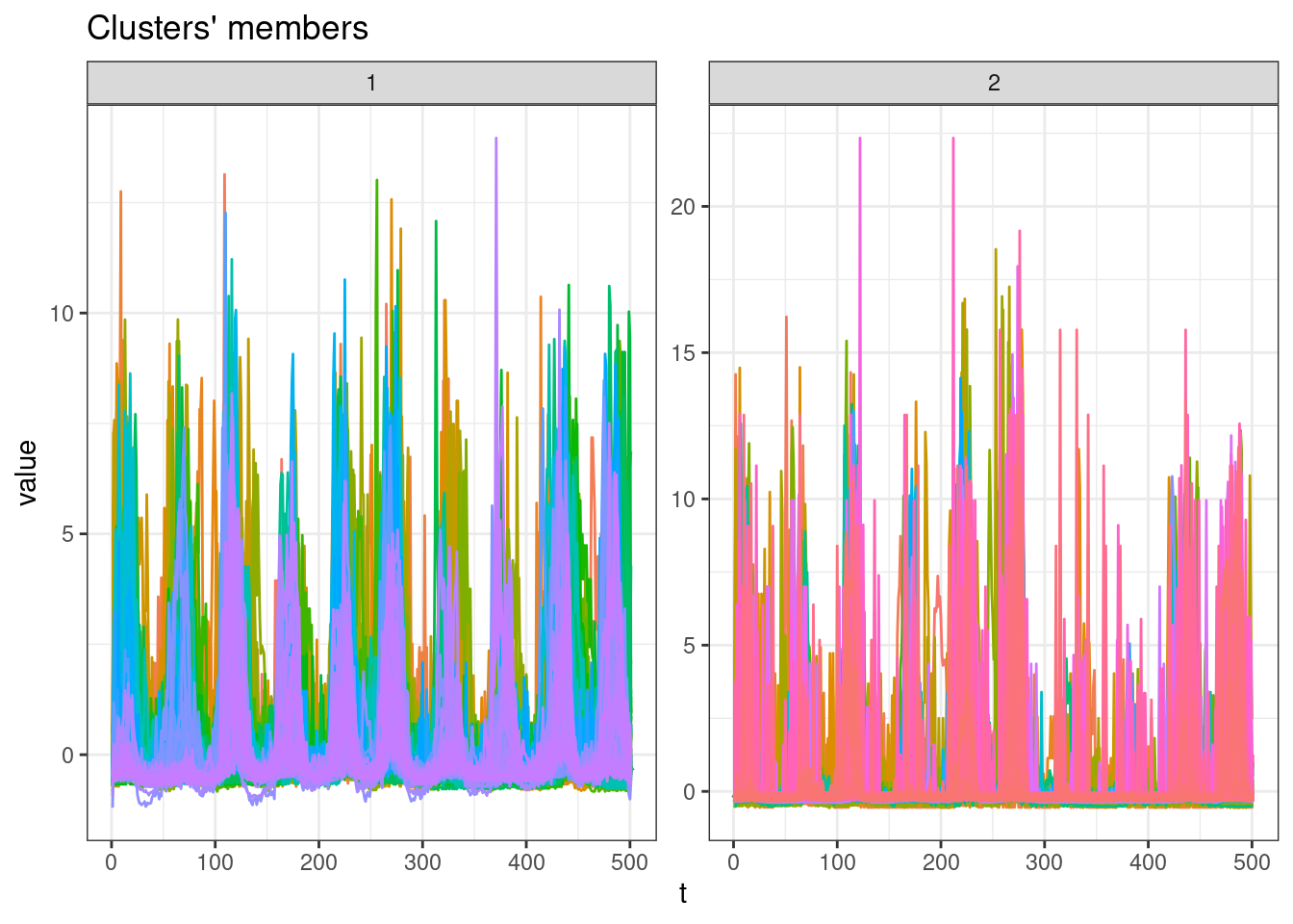

plot(sel_clust, type = "centroids", lty = 1)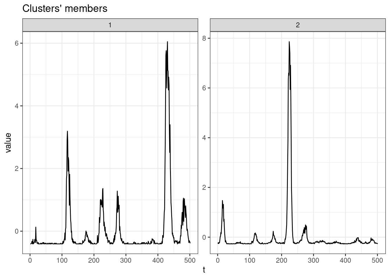

table(sel_clust@cluster)


  1   2 
292 387

Soft-DTW

tic()
clust_sdtw <- tsclust(
  series = tdengue, 
  type = "partitional", 
  k = k_seq,
  distance = "sdtw",
  seed = 13
)
toc()

204.708 sec elapsed

names(clust_sdtw) <- paste0("k_", k_seq)
res_cvi <- sapply(clust_sdtw, cvi, type = "internal") %>% 
  t() %>%
  as_tibble(rownames = "k") %>%
  arrange(-Sil)

res_cvi %>%
  gt::gt()

k	Sil	CH	DB	DBstar	D	COP
k_2	0.54420550	424.7128	1.784989	1.784989	0.0188267923	0.2699432
k_6	0.23058175	150.9456	1.252811	1.660076	0.0056554246	0.1492226
k_5	0.20100983	179.4794	2.019992	3.279759	0.0062697286	0.1565015
k_4	0.16735749	197.7269	2.204787	5.000366	0.0014544262	0.1900948
k_3	0.16612027	203.6722	4.148653	4.660288	0.0095083455	0.2259238
k_10	0.14175838	106.8324	1.978932	3.094434	0.0079666165	0.1331531
k_7	0.13487754	136.8319	1.860672	3.131776	-0.0017931128	0.1454316
k_9	0.11776105	106.7446	2.427594	4.376014	-0.0082114090	0.1384285
k_8	0.07201448	121.5954	2.392449	5.993679	0.0005698678	0.1471381

sel_clust <- clust_sdtw[[res_cvi[[1,1]]]]

plot(sel_clust)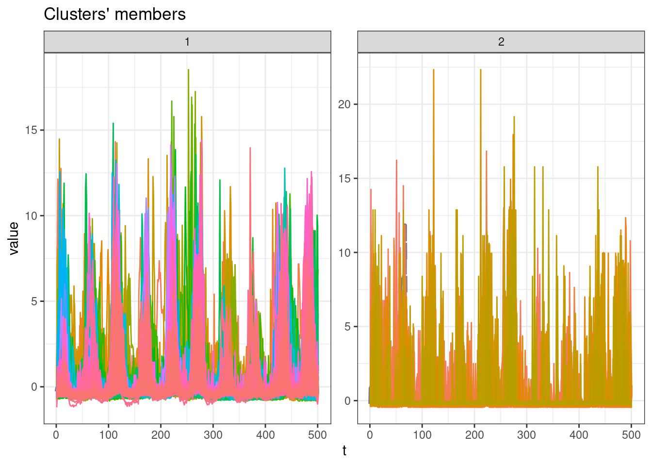

plot(sel_clust, type = "centroids", lty = 1)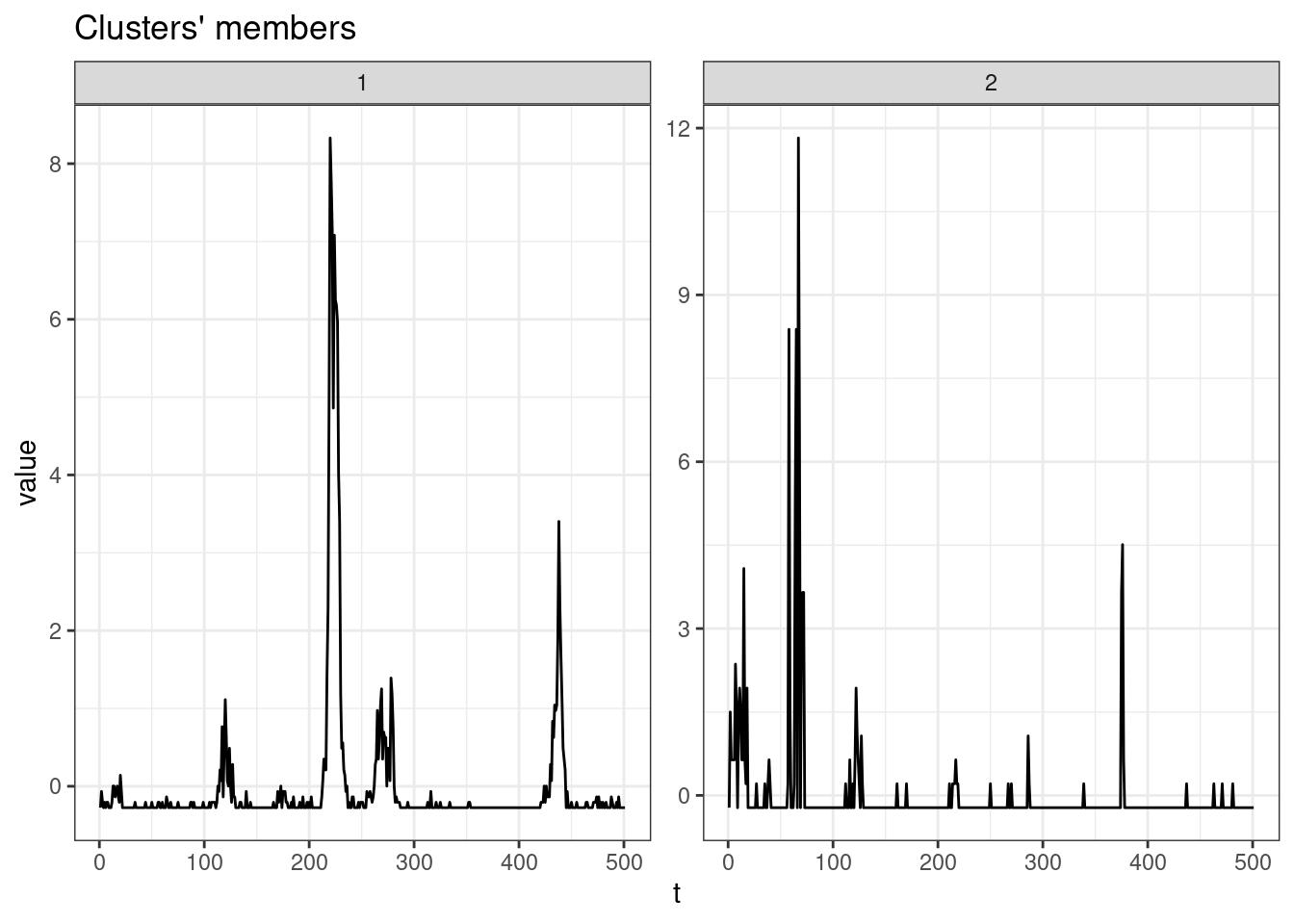

table(sel_clust@cluster)


  1   2 
581  98

SBD

tic()
clust_sbd <- tsclust(
  series = tdengue, 
  type = "partitional", 
  k = k_seq,
  distance = "sbd",
  seed = 13
)
toc()

0.792 sec elapsed

names(clust_sbd) <- paste0("k_", k_seq)
res_cvi <- sapply(clust_sbd, cvi, type = "internal") %>% 
  t() %>%
  as_tibble(rownames = "k") %>%
  arrange(-Sil)

res_cvi %>%
  gt::gt()

k	Sil	SF	CH	DB	DBstar	D	COP
k_2	0.19153388	0.41954595	92.48199	4.965541	4.965541	0.05215726	0.3986087
k_6	0.17383693	0.15654880	45.49664	3.416220	3.694440	0.09627307	0.3700479
k_5	0.15090087	0.16086274	51.05856	2.100628	2.794277	0.08129365	0.3596084
k_10	0.09507187	0.03507591	37.49864	2.666277	3.750657	0.05350097	0.3320909
k_8	0.07435107	0.07700081	29.71794	4.390497	6.258006	0.04658001	0.3447000
k_9	0.05379396	0.05994618	39.01541	3.867380	5.360924	0.03345584	0.3376868
k_7	0.03260668	0.10548796	48.66182	4.096509	5.928294	0.02534005	0.3453233
k_3	0.02929865	0.29847866	58.62624	5.033205	6.498922	0.02115696	0.3885022
k_4	0.02545150	0.23112470	50.67983	5.198919	6.670280	0.02116725	0.3814808

sel_clust <- clust_sbd[[res_cvi[[1,1]]]]

plot(sel_clust)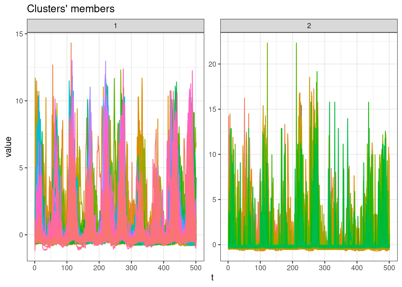

plot(sel_clust, type = "centroids", lty = 1)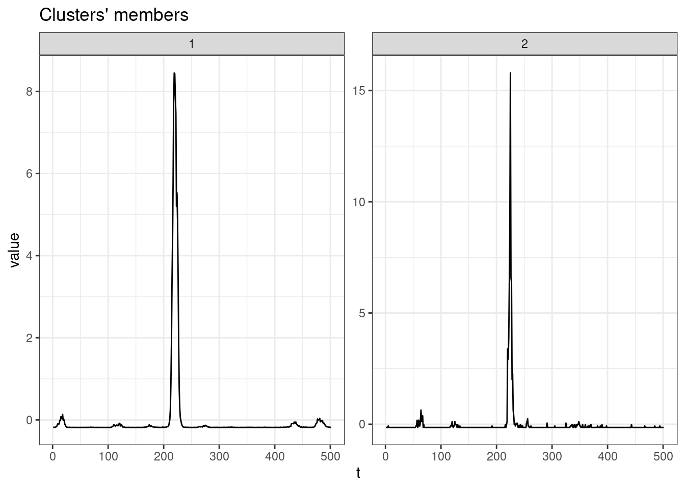

table(sel_clust@cluster)


  1   2 
503 176

GAK

tic()
clust_gak <- tsclust(
  series = tdengue, 
  type = "partitional", 
  k = k_seq,
  distance = "gak",
  seed = 13
)
toc()

260.459 sec elapsed

names(clust_gak) <- paste0("k_", k_seq)
res_cvi <- sapply(clust_gak, cvi, type = "internal") %>% 
  t() %>%
  as_tibble(rownames = "k") %>%
  arrange(-Sil)

res_cvi %>%
  gt::gt()

k	Sil	SF	CH	DB	DBstar	D	COP
k_6	0.2830846	0.6304283	124.45464	2.229032	2.350710	0.009648476	0.2459049
k_9	0.2591976	0.6297937	102.39058	2.243505	3.344258	0.007771500	0.2020673
k_7	0.2559452	0.6301835	105.07795	2.610798	2.716722	0.009410867	0.2473205
k_10	0.2550581	0.6295251	95.02169	2.043610	2.248546	0.008625614	0.1991254
k_5	0.2253127	0.6305288	110.82437	1.737232	1.904585	0.008938342	0.3000306
k_3	0.1974647	0.6309581	98.32655	3.945344	4.077690	0.006170275	0.3651774
k_8	0.1823244	0.6298506	74.98460	2.864885	2.987567	0.010215175	0.2561144
k_2	0.1584990	0.6314929	203.86335	2.899706	2.899706	0.020554844	0.5280049
k_4	0.1423961	0.6306801	101.83124	3.970774	4.082930	0.005129007	0.3477263

sel_clust <- clust_gak[[res_cvi[[1,1]]]]

plot(sel_clust)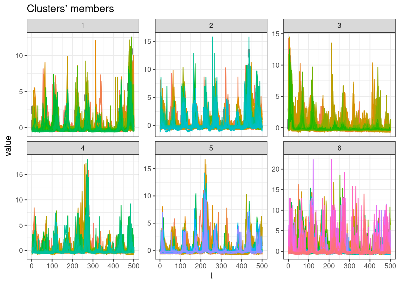

plot(sel_clust, type = "centroids", lty = 1)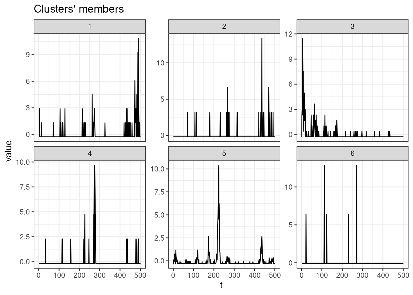

table(sel_clust@cluster)


  1   2   3   4   5   6 
 73 104  64  91 144 203

Session info

sessionInfo()

R version 4.3.2 (2023-10-31)
Platform: x86_64-pc-linux-gnu (64-bit)
Running under: Ubuntu 22.04.3 LTS

Matrix products: default
BLAS:   /usr/lib/x86_64-linux-gnu/blas/libblas.so.3.10.0 
LAPACK: /usr/lib/x86_64-linux-gnu/lapack/liblapack.so.3.10.0

Random number generation:
 RNG:     L'Ecuyer-CMRG 
 Normal:  Inversion 
 Sample:  Rejection 
 
locale:
 [1] LC_CTYPE=en_US.UTF-8       LC_NUMERIC=C              
 [3] LC_TIME=en_CA.UTF-8        LC_COLLATE=en_US.UTF-8    
 [5] LC_MONETARY=en_CA.UTF-8    LC_MESSAGES=en_US.UTF-8   
 [7] LC_PAPER=en_CA.UTF-8       LC_NAME=C                 
 [9] LC_ADDRESS=C               LC_TELEPHONE=C            
[11] LC_MEASUREMENT=en_CA.UTF-8 LC_IDENTIFICATION=C       

time zone: Europe/Paris
tzcode source: system (glibc)

attached base packages:
[1] stats     graphics  grDevices utils     datasets  methods   base     

other attached packages:
 [1] tictoc_1.2       kableExtra_1.3.4 dtwclust_5.5.12  dtw_1.23-1      
 [5] proxy_0.4-27     timetk_2.9.0     arrow_13.0.0.1   lubridate_1.9.3 
 [9] forcats_1.0.0    stringr_1.5.0    dplyr_1.1.3      purrr_1.0.2     
[13] readr_2.1.4      tidyr_1.3.0      tibble_3.2.1     ggplot2_3.4.4   
[17] tidyverse_2.0.0 

loaded via a namespace (and not attached):
  [1] rlang_1.1.2         magrittr_2.0.3      clue_0.3-65        
  [4] furrr_0.3.1         flexclust_1.4-1     compiler_4.3.2     
  [7] systemfonts_1.0.5   vctrs_0.6.4         reshape2_1.4.4     
 [10] rvest_1.0.3         lhs_1.1.6           tune_1.1.2         
 [13] pkgconfig_2.0.3     fastmap_1.1.1       ellipsis_0.3.2     
 [16] labeling_0.4.3      utf8_1.2.4          promises_1.2.1     
 [19] rmarkdown_2.25      prodlim_2023.08.28  tzdb_0.4.0         
 [22] bit_4.0.5           xfun_0.41           modeltools_0.2-23  
 [25] jsonlite_1.8.7      recipes_1.0.8       later_1.3.1        
 [28] parallel_4.3.2      cluster_2.1.4       R6_2.5.1           
 [31] stringi_1.7.12      rsample_1.2.0       parallelly_1.36.0  
 [34] rpart_4.1.21        Rcpp_1.0.11         assertthat_0.2.1   
 [37] dials_1.2.0         iterators_1.0.14    knitr_1.45         
 [40] future.apply_1.11.0 zoo_1.8-12          httpuv_1.6.12      
 [43] Matrix_1.6-1.1      splines_4.3.2       nnet_7.3-19        
 [46] timechange_0.2.0    tidyselect_1.2.0    rstudioapi_0.15.0  
 [49] yaml_2.3.7          timeDate_4022.108   codetools_0.2-19   
 [52] listenv_0.9.0       lattice_0.22-5      plyr_1.8.9         
 [55] shiny_1.7.5.1       withr_2.5.2         evaluate_0.23      
 [58] future_1.33.0       survival_3.5-7      RcppParallel_5.1.7 
 [61] xml2_1.3.5          xts_0.13.1          pillar_1.9.0       
 [64] foreach_1.5.2       stats4_4.3.2        shinyjs_2.1.0      
 [67] generics_0.1.3      hms_1.1.3           munsell_0.5.0      
 [70] scales_1.2.1        xtable_1.8-4        globals_0.16.2     
 [73] class_7.3-22        glue_1.6.2          tools_4.3.2        
 [76] data.table_1.14.8   RSpectra_0.16-1     webshot_0.5.5      
 [79] gower_1.0.1         grid_4.3.2          yardstick_1.2.0    
 [82] ipred_0.9-14        colorspace_2.1-0    cli_3.6.1          
 [85] DiceDesign_1.9      workflows_1.1.3     parsnip_1.1.1      
 [88] fansi_1.0.5         viridisLite_0.4.2   gt_0.10.0          
 [91] svglite_2.1.2       lava_1.7.3          gtable_0.3.4       
 [94] GPfit_1.0-8         sass_0.4.7          digest_0.6.33      
 [97] ggrepel_0.9.4       farver_2.1.1        htmlwidgets_1.6.2  
[100] htmltools_0.5.7     lifecycle_1.0.4     httr_1.4.7         
[103] hardhat_1.3.0       mime_0.12           bit64_4.0.5        
[106] MASS_7.3-60